ISOFIT Atmospheric Correction — Arizona Area Trial
Scene Footprints
Geographic footprints of all 23 EMIT scenes used in this whitepaper, colored by the shared gta_quality tier. Click any footprint for its scene ID and QC reason; use the sliders to adjust per-tier fill opacity.
Abstract: The Imaging Spectrometer Optimal FITting (ISOFIT) framework solves the coupled surface–atmosphere inverse problem from at-sensor radiance, retrieving per-pixel surface reflectance simultaneously with atmospheric water vapor and aerosol optical thickness via Accelerated Optimal Estimation. We summarize the algorithm and present a side-by-side comparison of the JPL operational EMIT L2A V001 product against a local ISOFIT + sRTMnet retrieval on 23 EMIT scenes covering Arizona Area Trial. For each scene we provide a true-color RGB pair with PC-pure pixel markers, mean and selected spectra, the first eighteen principal-component composites, the eigenvalue spectrum, and a nested mineral-spectral-index accordion.
1. Why Atmospheric Correction Matters
An imaging spectrometer measures at-sensor radiance \(L(\lambda)\) — a tangled superposition of light scattered by atmospheric molecules and aerosols, light reflected from the surface that transits the atmosphere twice, and the spherical-albedo coupling between the two. Recovering surface reflectance \(\rho(\lambda)\) requires inverting that radiative transfer chain pixel-by-pixel.
The algorithms here apply to a family of NASA imaging spectrometers — AVIRIS-Classic, AVIRIS-NG, AVIRIS-3, and EMIT — that share a common forward-model architecture in ISOFIT. The 23 scenes presented here come from EMIT.
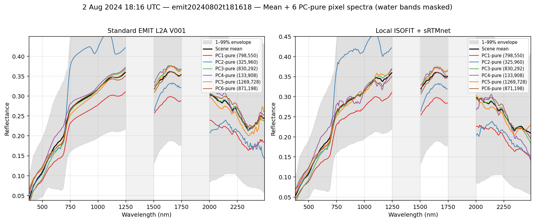
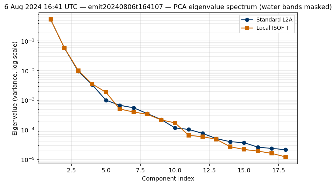
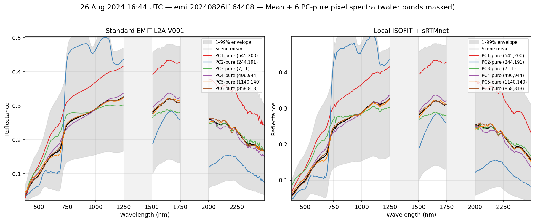
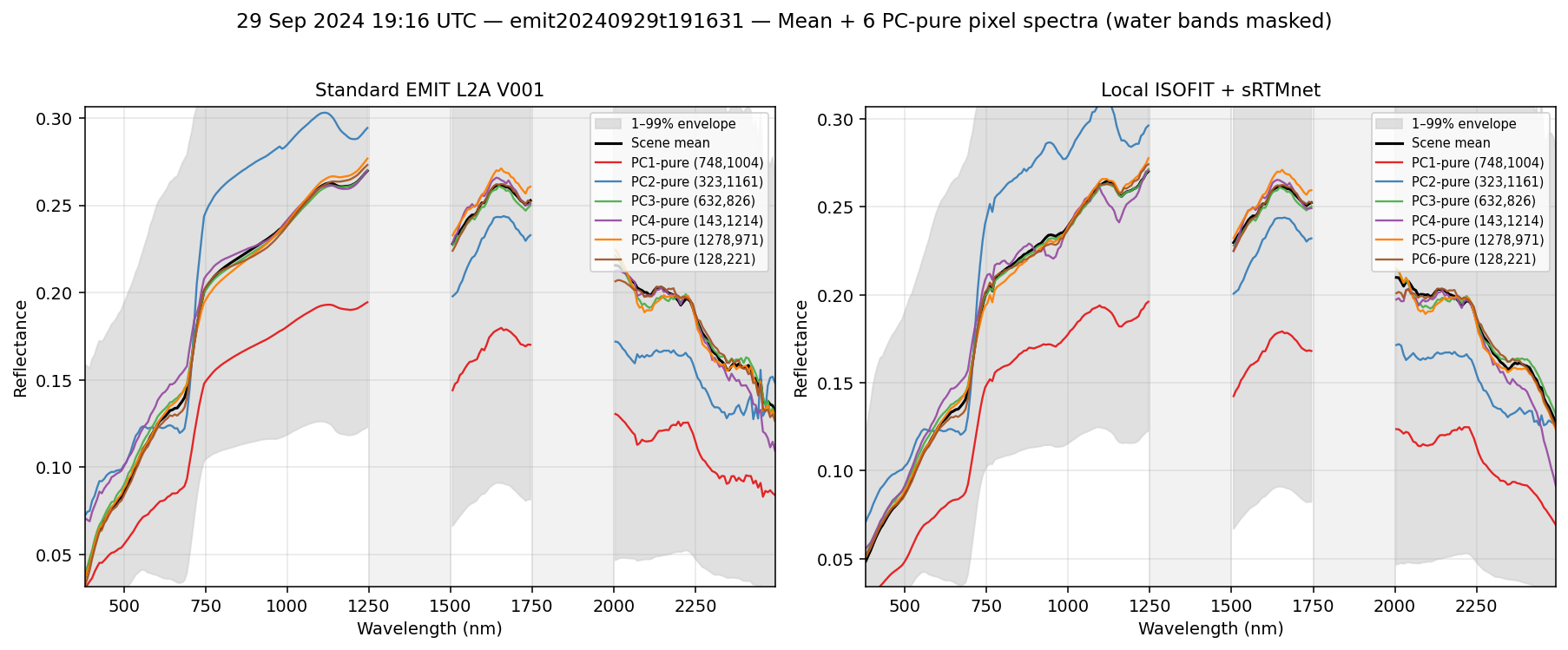
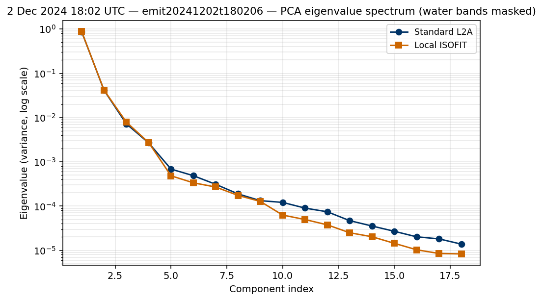
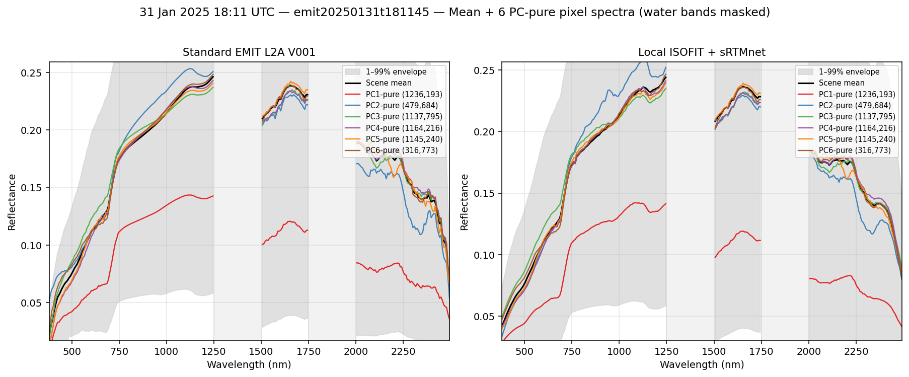
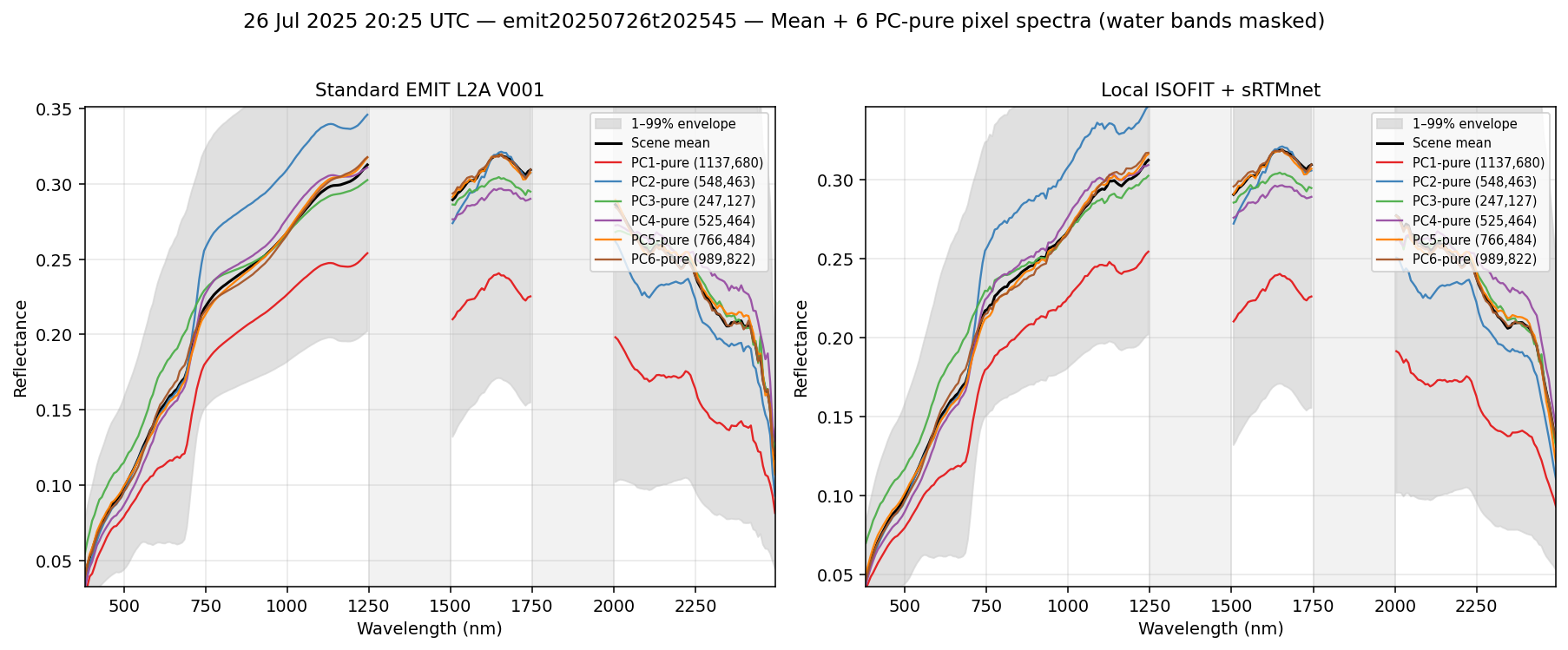
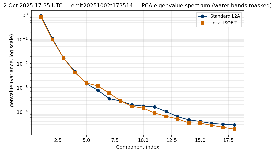
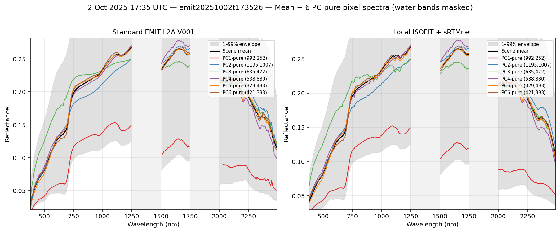
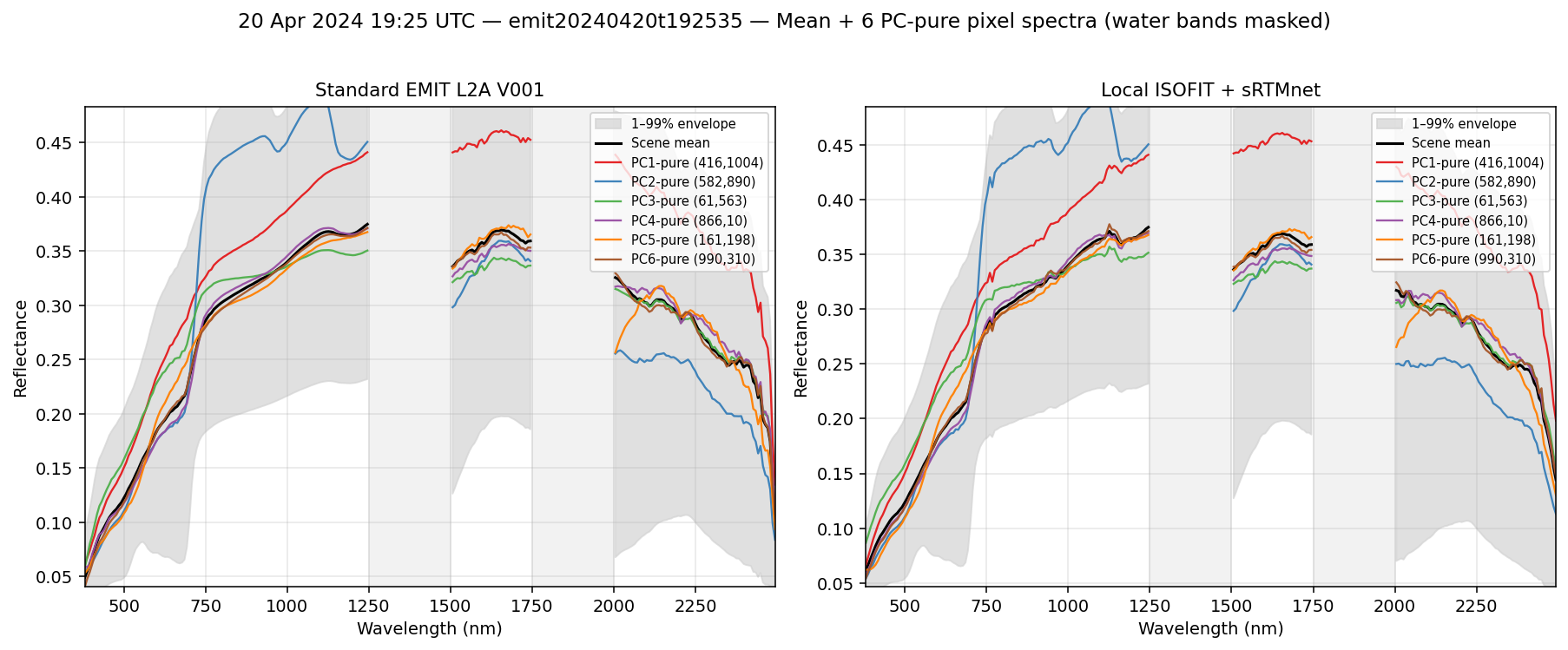
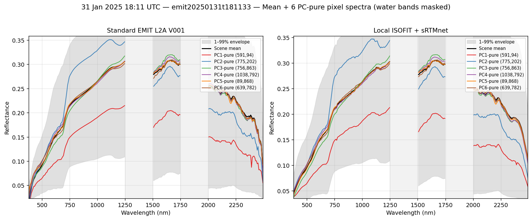
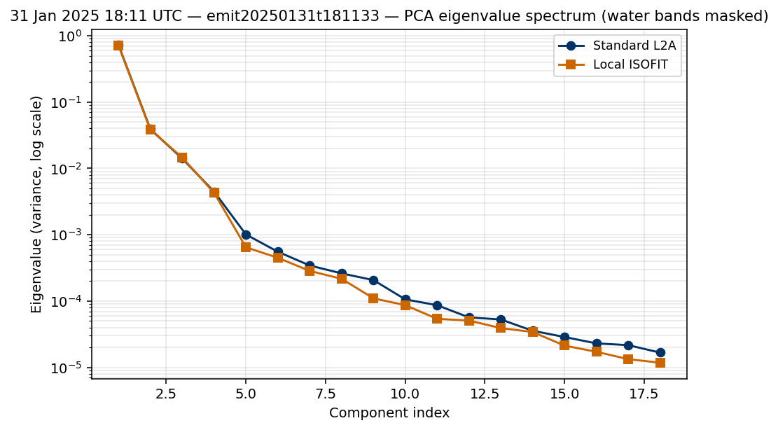
Two atmospheric water-vapor absorption regions, 1250–1500 nm and
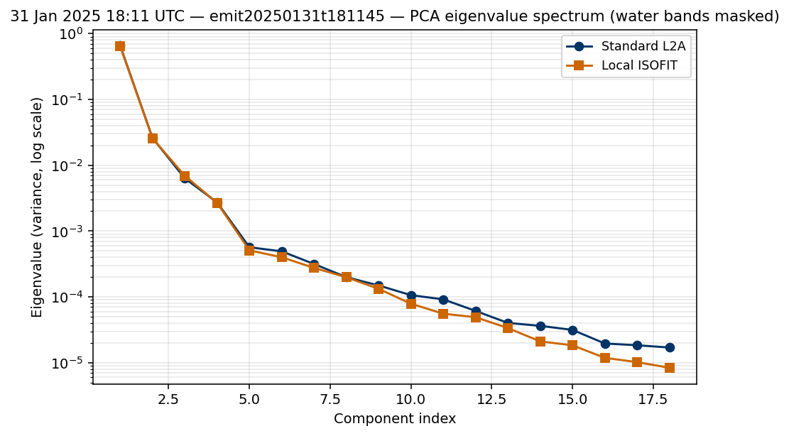
1750–2000 nm, are explicitly excluded from PCA fitting, the
eigenvalue spectrum, the ASTER-band synthesis used for the mineral indices,
and the spectra plots (where the lines visibly break across those windows).
The masks are applied in addition to the per-pixel band-quality flags
(bbl) embedded in each retrieval. This isolates the comparison from
the wavelengths most contaminated by atmospheric residuals — keeping the
principal-component structure dominated by surface variance rather than
unconverged H₂O absorption.
2. The ISOFIT Algorithm
2.1 The Forward Model
ISOFIT writes the at-sensor radiance as the composition of a surface model \(\rho(\mathbf{x}_s; \lambda)\) and an atmosphere model \(\mathcal{A}(\mathbf{x}_a; \lambda)\):
where \(\mathbf{R}\) applies the spectral response of the instrument and \(\mathbf{x}_s\), \(\mathbf{x}_a\) are the surface- and atmospheric-state vectors. The state \(\mathbf{x}_a\) is kept low-dimensional (column water vapor, AOT at 550 nm) because well-mixed gases can be held at climatology with negligible error in retrieved \(\rho\).
2.2 Accelerated Optimal Estimation
OE inverts the forward model under a Gaussian prior and Gaussian instrument noise. The cost is:
The Accelerated formulation collapses the >280-dimensional Levenberg–Marquardt iteration into a closed-form surface inversion wrapped in a small two-dimensional outer search over the atmospheric state, so retrievals are orders of magnitude faster while still reporting a full posterior covariance.
2.3 Radiative Transfer Engines and sRTMnet
The forward model needs \(\{L_a, T_\downarrow T_\uparrow, s\}\) at every wavelength for every plausible atmospheric state. ISOFIT supports MODTRAN 6 (operational JPL reference), LibRadTran (open-source), 6S (open-source, fast), and sRTMnet, a deep neural emulator trained on millions of 6S calls. We use sRTMnet for both EMIT and AVIRIS pipelines.
2.4 The Multicomponent Surface Prior
Without a prior, OE on a 285-channel reflectance spectrum is ill-posed. The multicomponent surface model partitions a global reflectance training set (vegetation, soils, water, mineral surfaces, snow) by k-means and assigns a Gaussian prior to each cluster; per pixel, ISOFIT picks the most likely component from a radiance-domain pre-classification, then uses that component's prior in the OE inversion.
3. The "Standard" Reflectance We Compare Against
We compare to the official EMIT L2A surface reflectance product as distributed by NASA's LP DAAC. Each scene's NetCDF header records its provenance:
title:        EMIT L2A Estimated Surface Reflectance 60 m V001
sensor:       EMIT (Earth Surface Mineral Dust Source Investigation)
platform:     ISS
institution:  NASA Jet Propulsion Laboratory / California Institute of Technology
software_build_version: 010621/010627
product_version: V001
The "standard" is the JPL operational ISOFIT pipeline (MODTRAN-based) running inside the EMIT Science Data System. Our local retrieval uses the open-source ISOFIT 3.7.x release with the sRTMnet neural emulator and a default multicomponent surface configuration:
description = L2A Analytical per-pixel surface retrieval
              (segmentation_size=40, engine=sRTMnet, isofit_version=3.7.x)
samples = 1242, lines = 1280, bands = 285
interleave = bil, no data value = -9999
Both retrievals operate on the same EMIT L1B radiance cube. Differences come from the radiative-transfer engine (full MODTRAN vs. sRTMnet emulator), the surface library configuration, and the segmentation size used to amortize OE across spatially coherent blocks.
4. Scene Comparisons 23 scenes
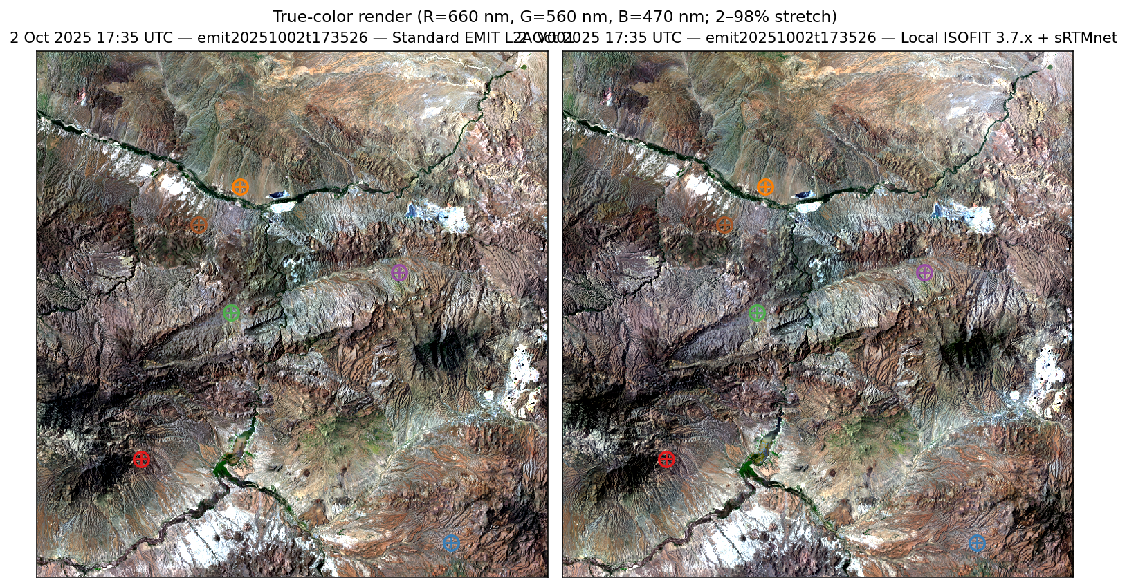
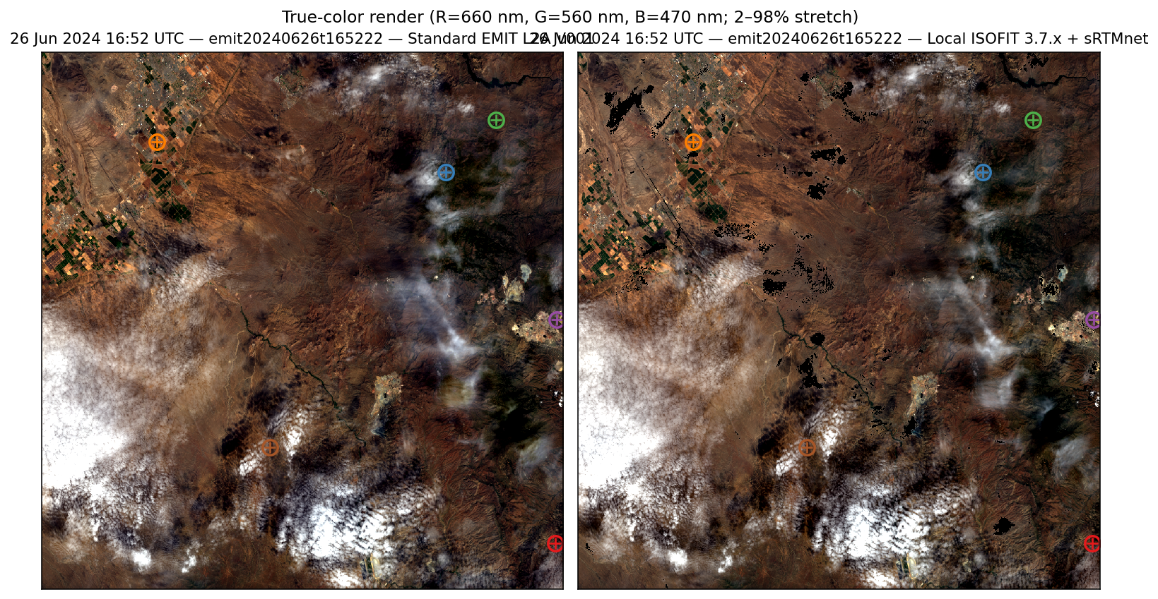
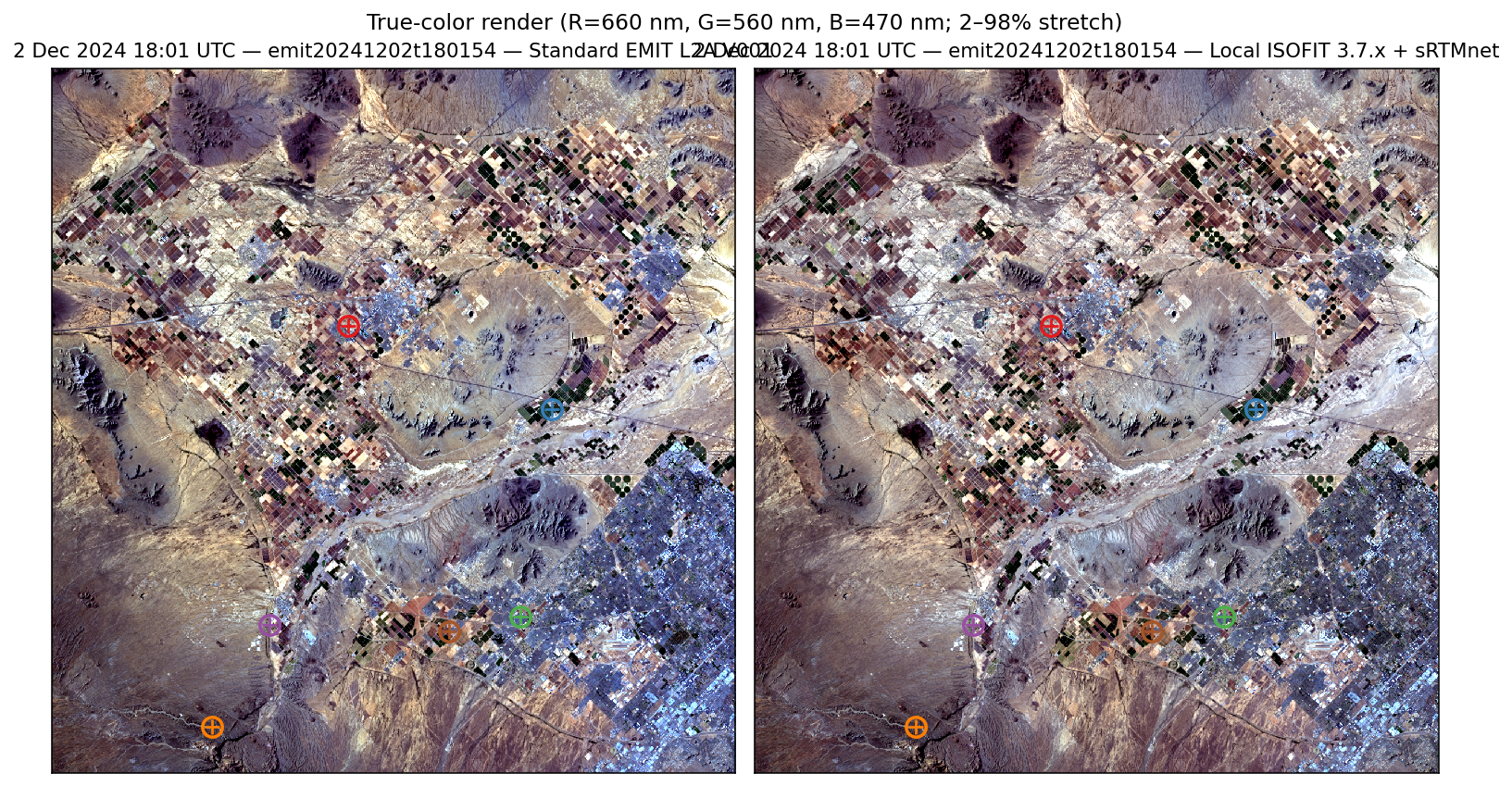
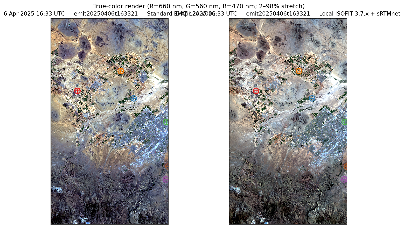
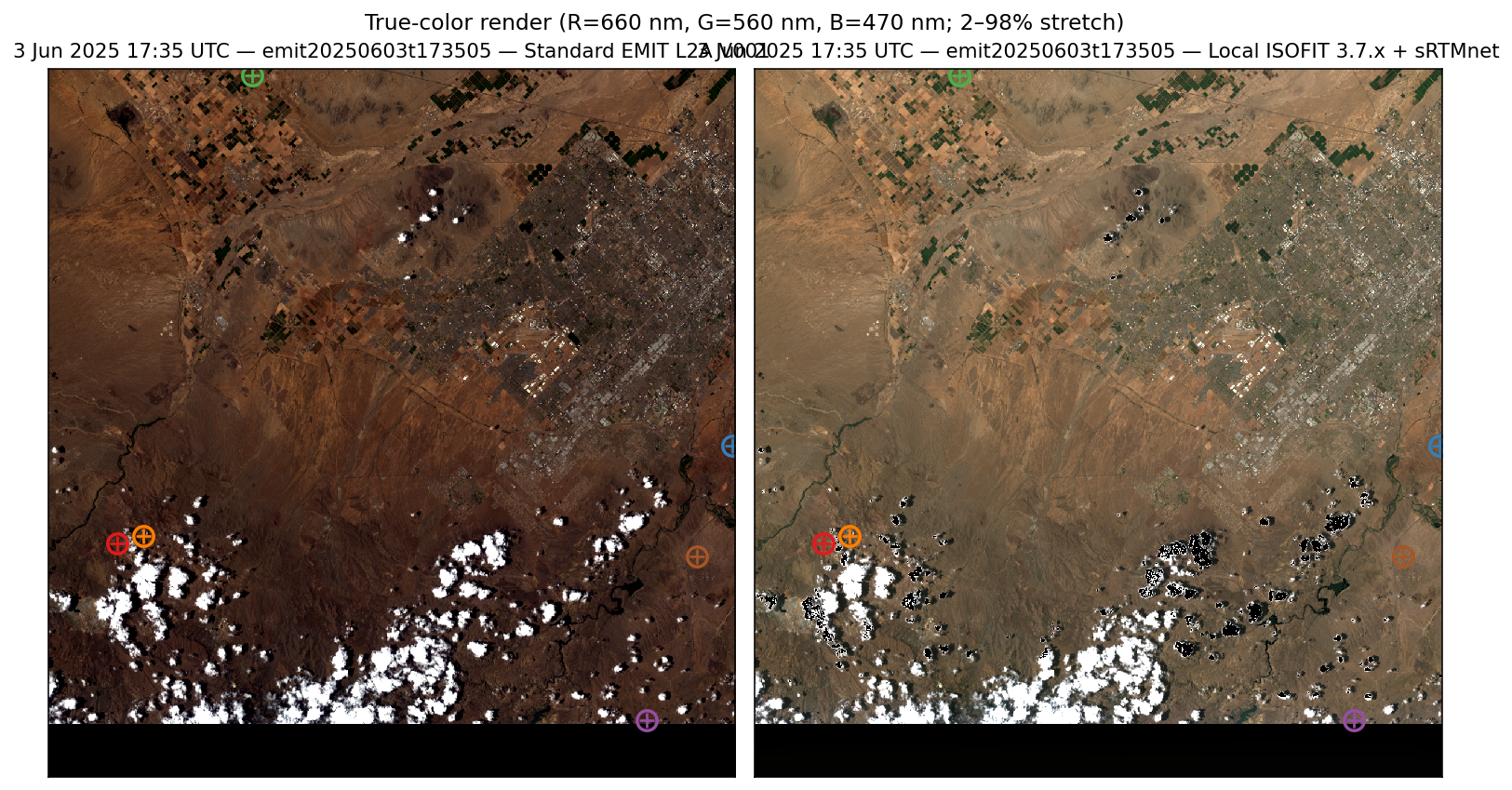
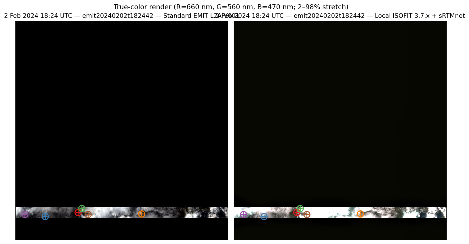
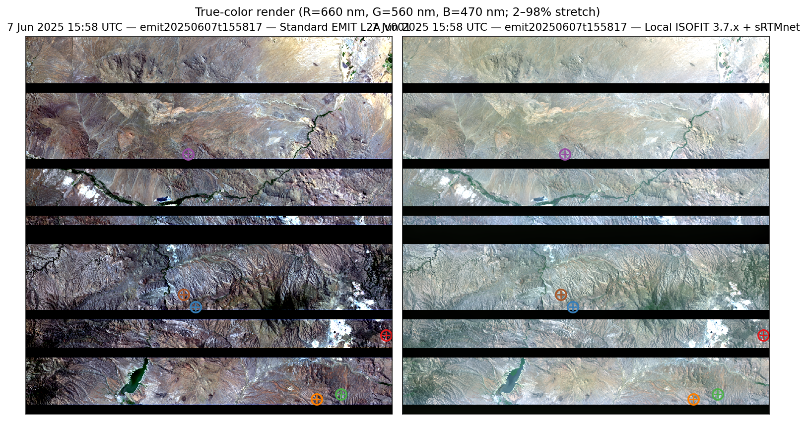
All 23 EMIT scenes are organized below by QC tier, following the Landsat Collection 2 convention: Tier 1 = best, Tier 4 = worst. Tier 1 (Excellent) and Tier 2 (Mild Cloud) scenes are processed and rendered with their full output set — RGB, spectra, PCA composites, eigenvalues, and the nested 15-map mineral-spectral-index accordion. Tier 3 (High Cloud) and Tier 4 (Missing Data) scenes are excluded from processing; only their RGB render is shown so you can see what was filtered. Click any processed scene to expand its full diagnostics; opening one collapses any other open scene.
| Scene | Tier | Dead rows | Cloud % | QC Notes |
|---|---|---|---|---|
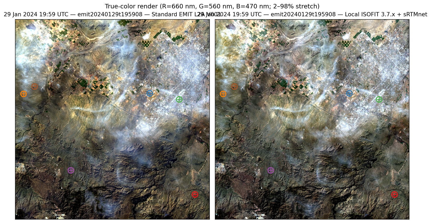
| 29 Jan 2024 19:59 UTC — emit20240129t195908 | T3 | 0.0% | 24.8% | cloud+cirrus+dilated = 24.8% (> 15%) |
| 2 Feb 2024 18:24 UTC — emit20240202t182442 | T4 | 95.0% | 100.0% | 95.0% dead rows (> 10%) |
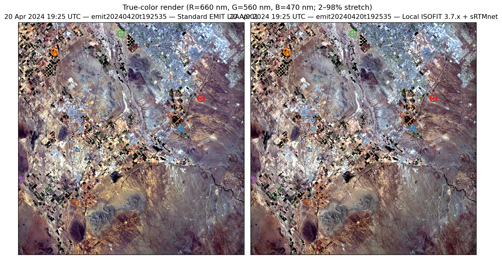
| 20 Apr 2024 19:25 UTC — emit20240420t192535 | T2 | 0.0% | 12.4% | cloud+cirrus+dilated = 12.4% (> 10%, ≤ 15%) |
| 20 Apr 2024 19:25 UTC — emit20240420t192547 | T2 | 0.0% | 11.8% | cloud+cirrus+dilated = 11.8% (> 10%, ≤ 15%) |
| 26 Jun 2024 16:52 UTC — emit20240626t165222 | T3 | 0.0% | 16.2% | cloud+cirrus+dilated = 16.2% (> 15%) |
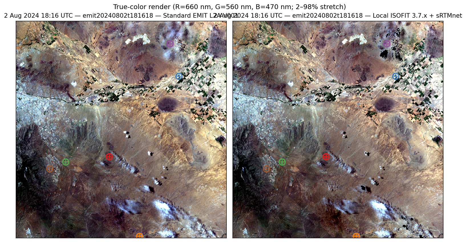
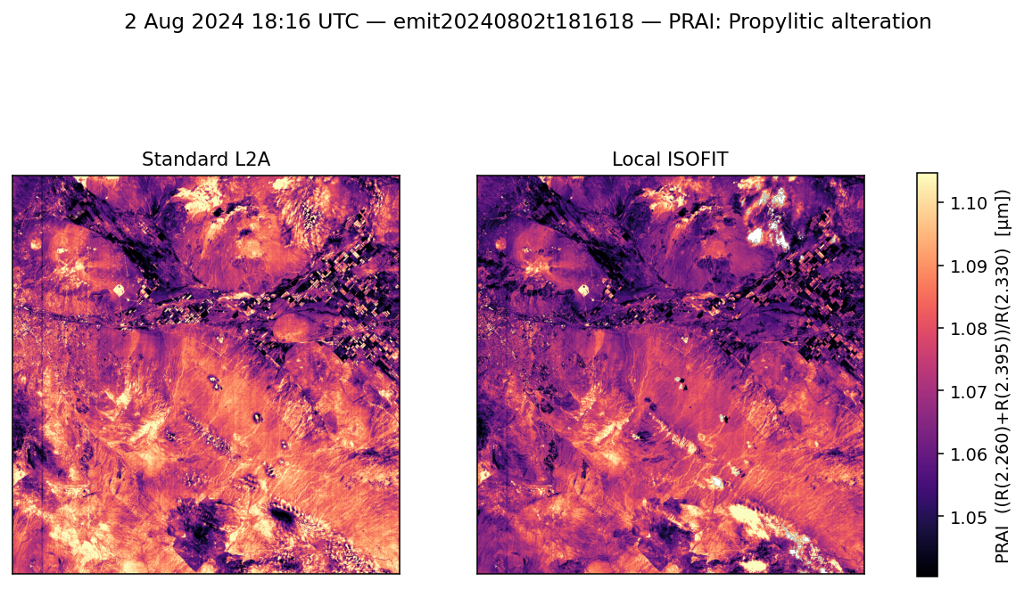
| 2 Aug 2024 18:16 UTC — emit20240802t181618 | T1 | 0.0% | 5.7% | all checks passed (cloud+cirrus+dilated = 5.7%) |
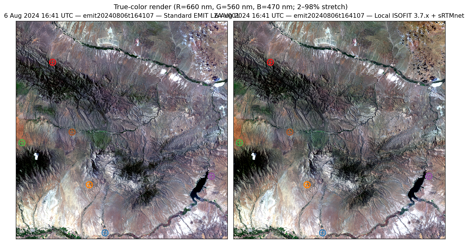
| 6 Aug 2024 16:41 UTC — emit20240806t164107 | T1 | 0.0% | 3.3% | all checks passed (cloud+cirrus+dilated = 3.3%) |
| 26 Aug 2024 16:44 UTC — emit20240826t164408 | T1 | 0.0% | 6.9% | all checks passed (cloud+cirrus+dilated = 6.9%) |
| 29 Sep 2024 19:16 UTC — emit20240929t191631 | T1 | 0.0% | 4.8% | all checks passed (cloud+cirrus+dilated = 4.8%) |
| 2 Dec 2024 18:01 UTC — emit20241202t180154 | T3 | 0.0% | 37.6% | cloud+cirrus+dilated = 37.6% (> 15%) |
| 2 Dec 2024 18:02 UTC — emit20241202t180206 | T1 | 0.0% | 8.8% | all checks passed (cloud+cirrus+dilated = 8.8%) |
| 31 Jan 2025 18:11 UTC — emit20250131t181133 | T2 | 0.0% | 14.1% | cloud+cirrus+dilated = 14.1% (> 10%, ≤ 15%) |
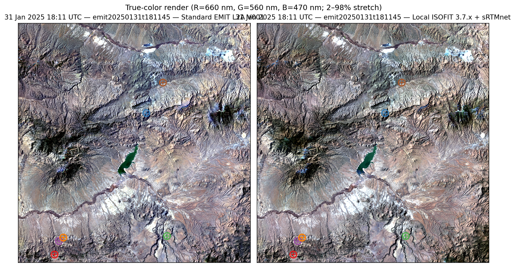
| 31 Jan 2025 18:11 UTC — emit20250131t181145 | T1 | 0.0% | 1.1% | all checks passed (cloud+cirrus+dilated = 1.1%) |
| 6 Apr 2025 16:33 UTC — emit20250406t163321 | T3 | 0.0% | 22.6% | cloud+cirrus+dilated = 22.6% (> 15%) |
| 3 Jun 2025 17:35 UTC — emit20250603t173505 | T3 | 7.5% | 44.3% | cloud+cirrus+dilated = 44.3% (> 15%) |
| 7 Jun 2025 15:58 UTC — emit20250607t155817 | T4 | 20.0% | 4.8% | interior gap(s) totaling 224 rows AND 20.0% dead rows (> 10%) |
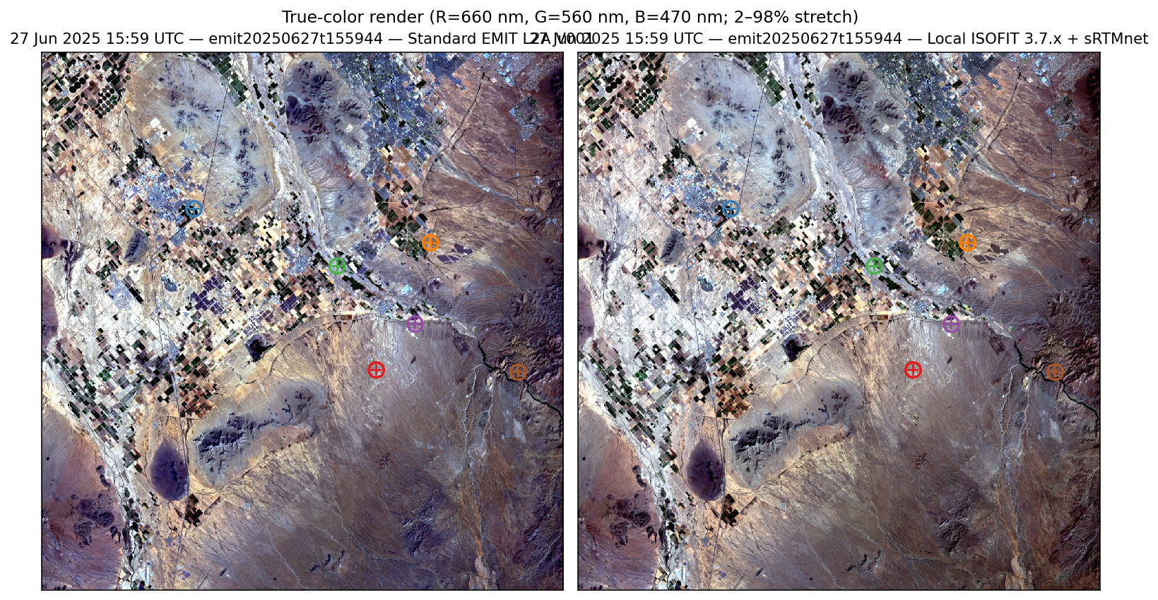
| 27 Jun 2025 15:59 UTC — emit20250627t155944 | T3 | 0.0% | 16.7% | cloud+cirrus+dilated = 16.7% (> 15%) |
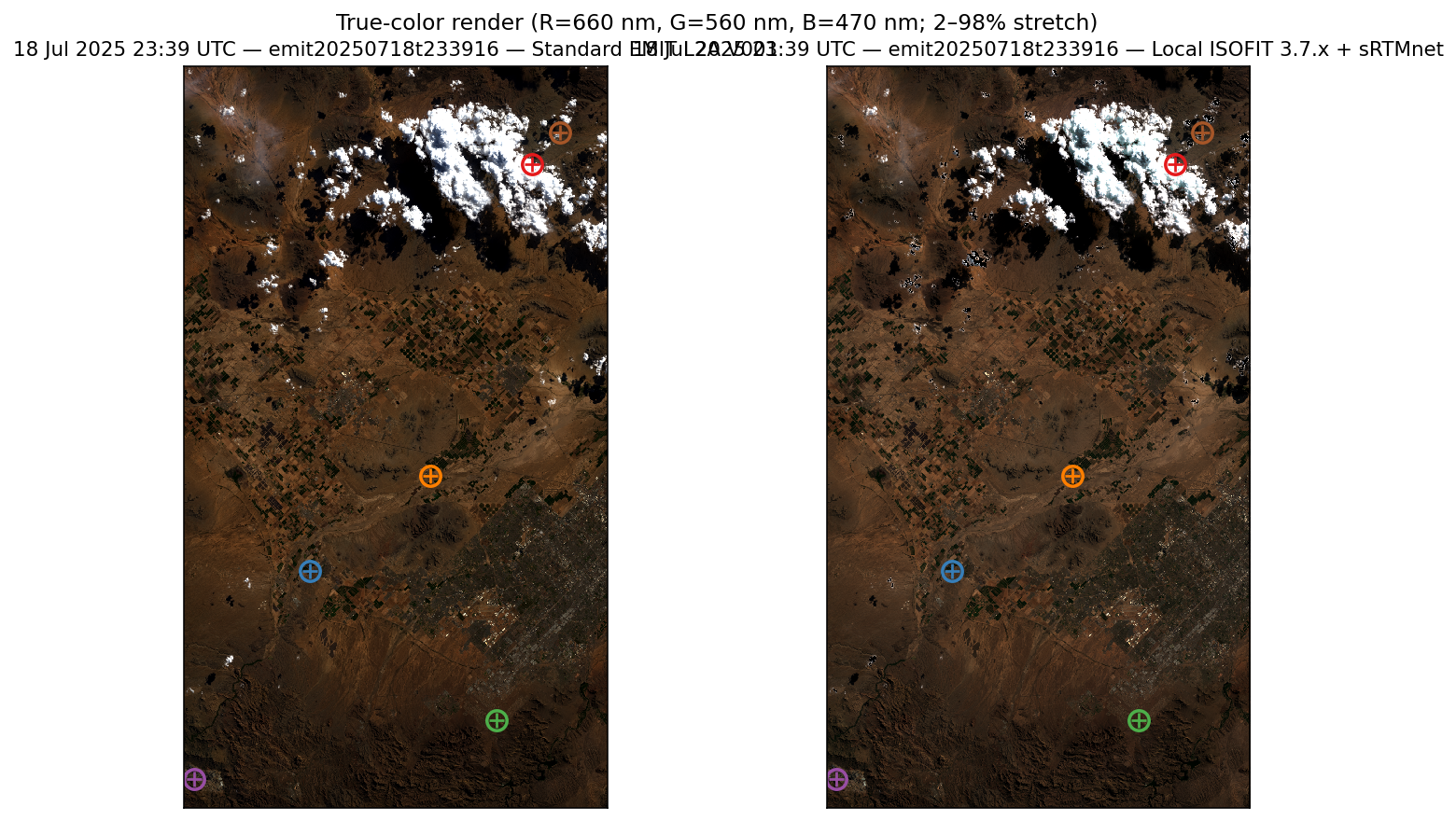
| 18 Jul 2025 23:39 UTC — emit20250718t233916 | T3 | 0.0% | 59.1% | cloud+cirrus+dilated = 59.1% (> 15%) |
| 26 Jul 2025 20:25 UTC — emit20250726t202545 | T1 | 0.0% | 0.1% | all checks passed (cloud+cirrus+dilated = 0.1%) |
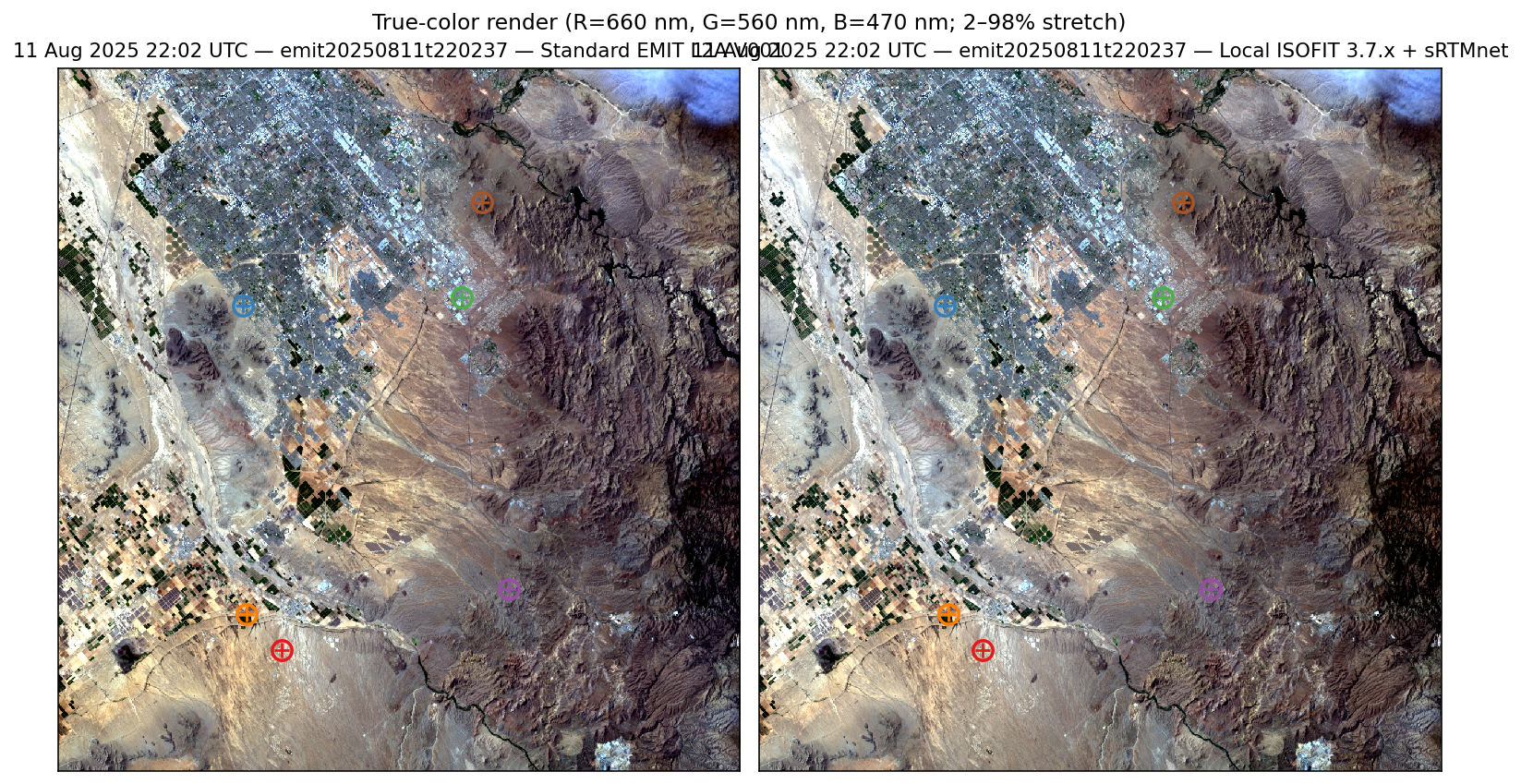
| 11 Aug 2025 22:02 UTC — emit20250811t220237 | T3 | 0.0% | 19.5% | cloud+cirrus+dilated = 19.5% (> 15%) |
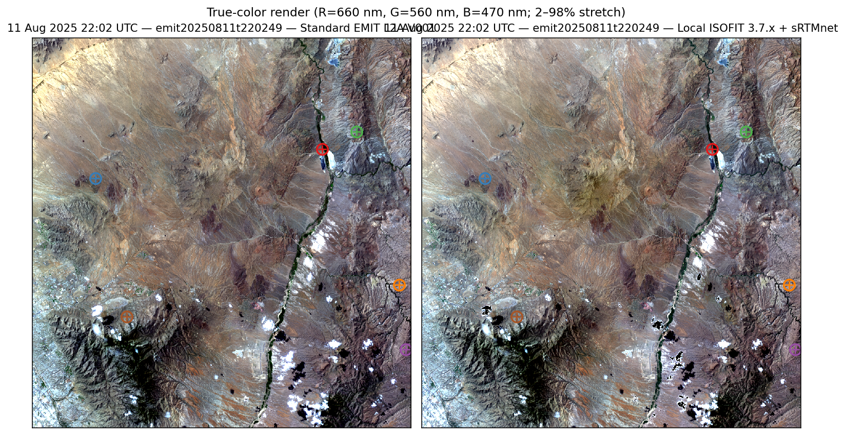
| 11 Aug 2025 22:02 UTC — emit20250811t220249 | T3 | 0.0% | 15.4% | cloud+cirrus+dilated = 15.4% (> 15%) |
| 2 Oct 2025 17:35 UTC — emit20251002t173514 | T1 | 0.0% | 9.2% | all checks passed (cloud+cirrus+dilated = 9.2%) |
| 2 Oct 2025 17:35 UTC — emit20251002t173526 | T1 | 0.0% | 2.0% | all checks passed (cloud+cirrus+dilated = 2.0%) |
Tier 1 — Excellent Quality Included in Processing 9 scenes
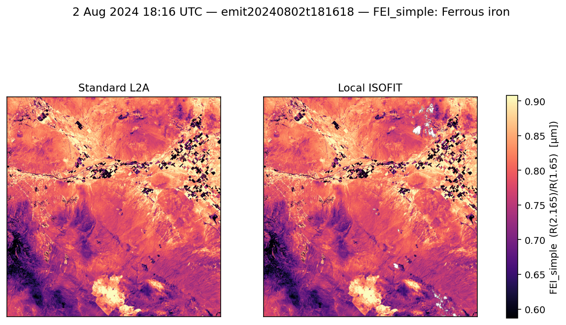
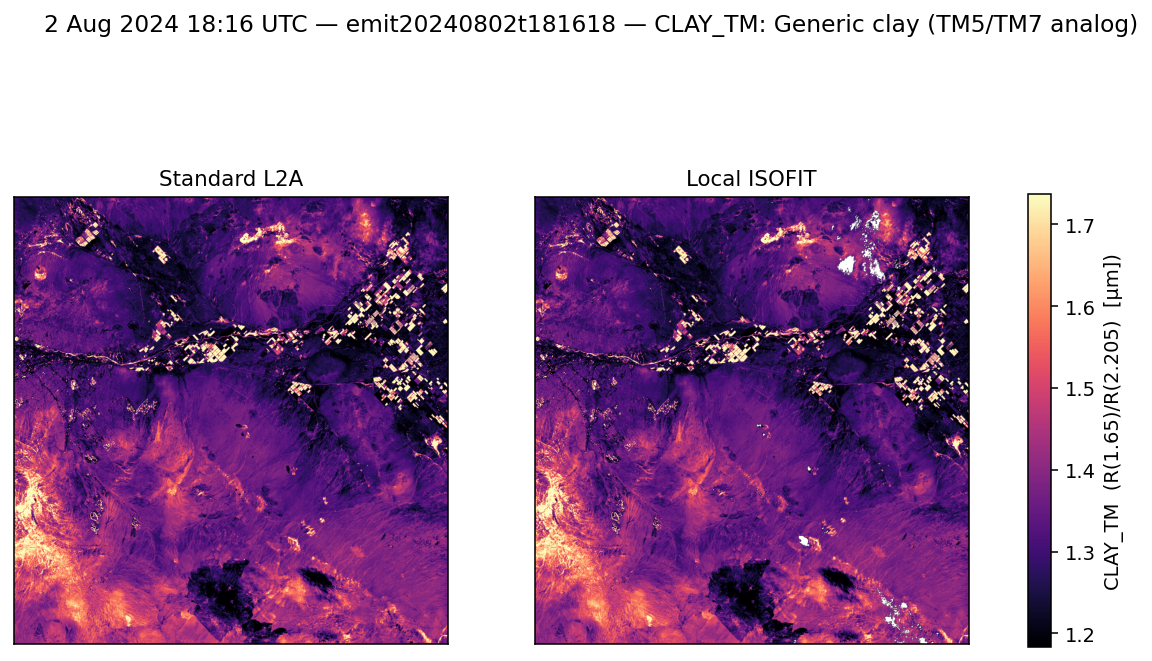
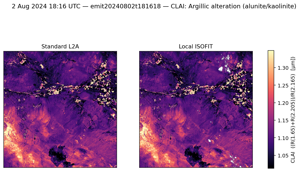
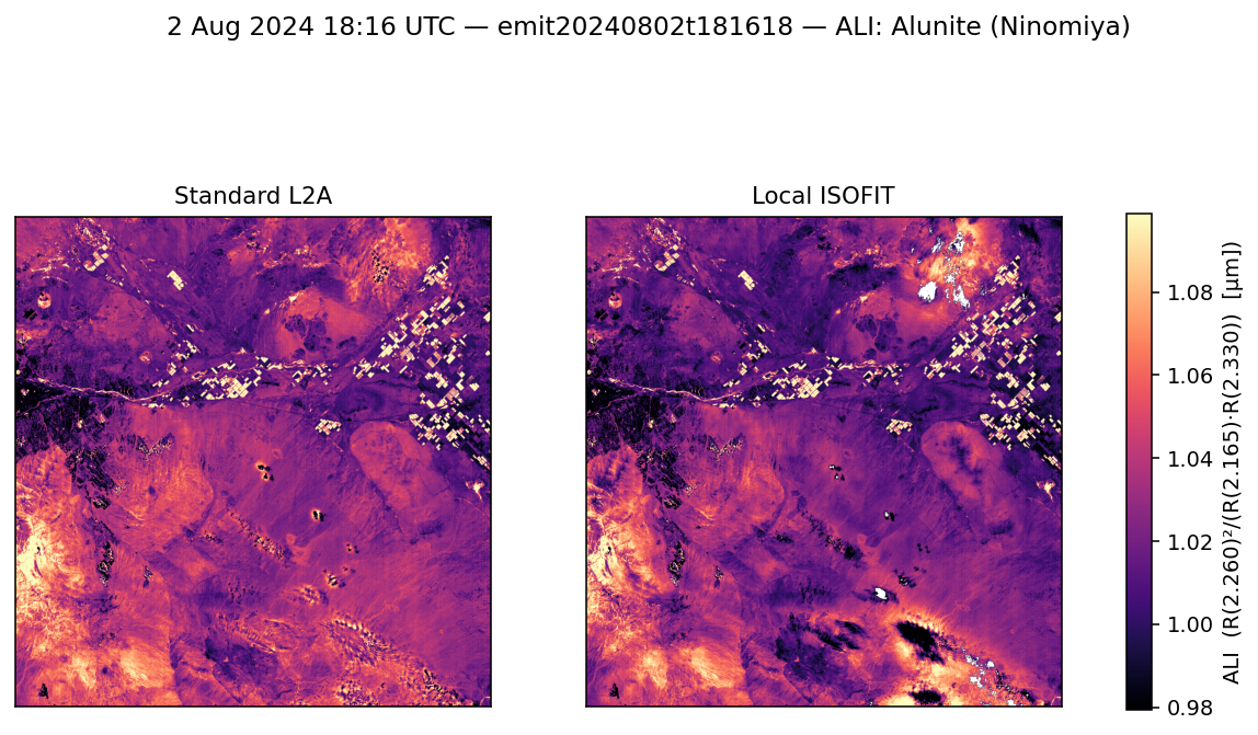
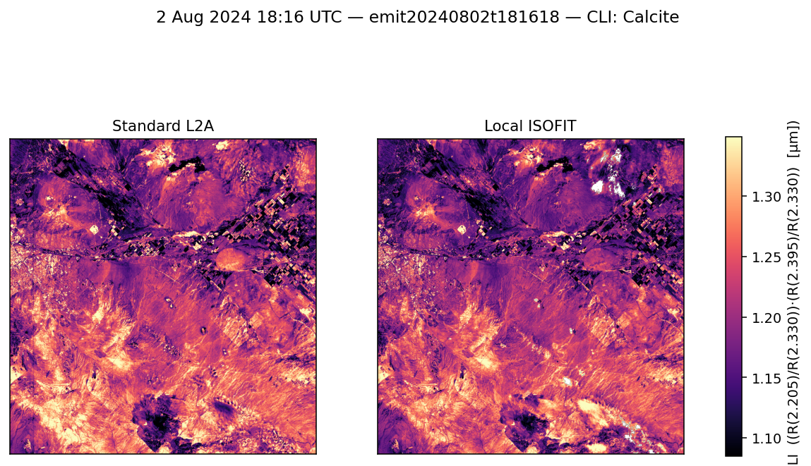
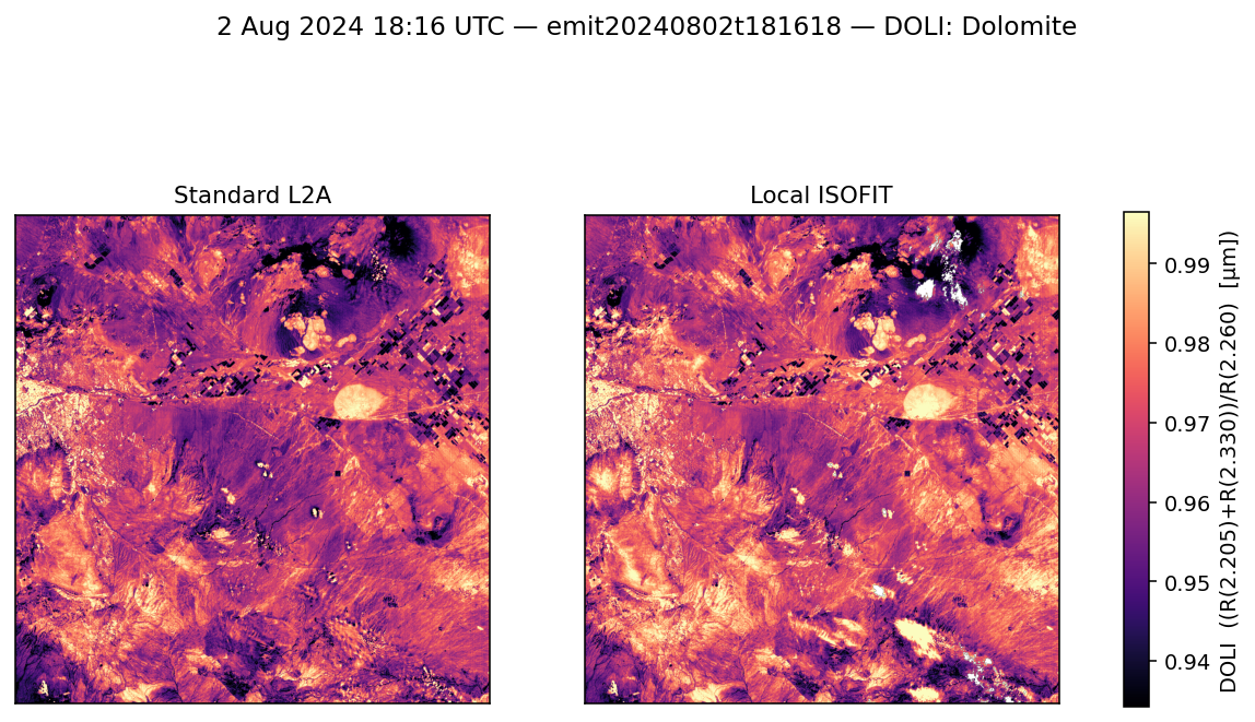
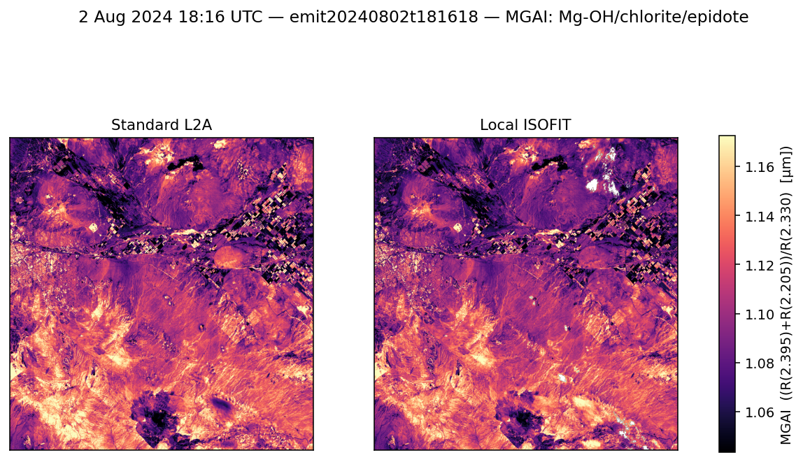
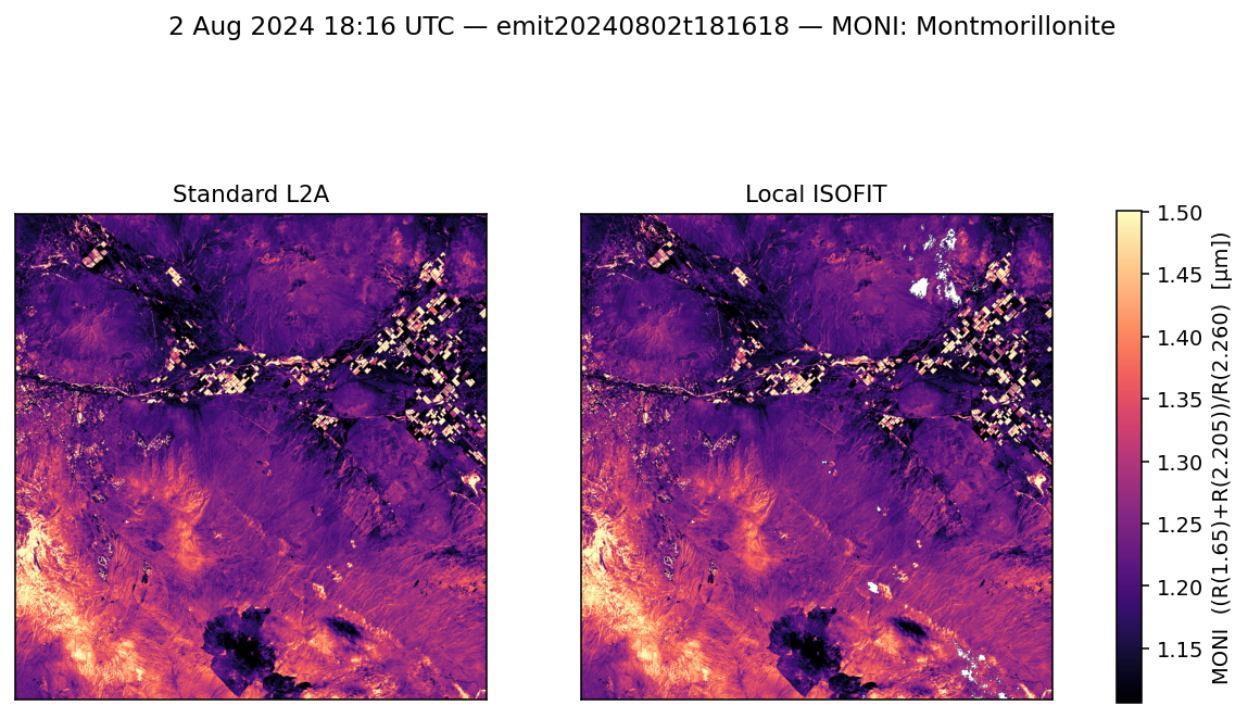
2 Aug 2024 18:16 UTC — emit20240802t181618
Click to expand spectra, PCA grid, eigenvalues, and mineral indices

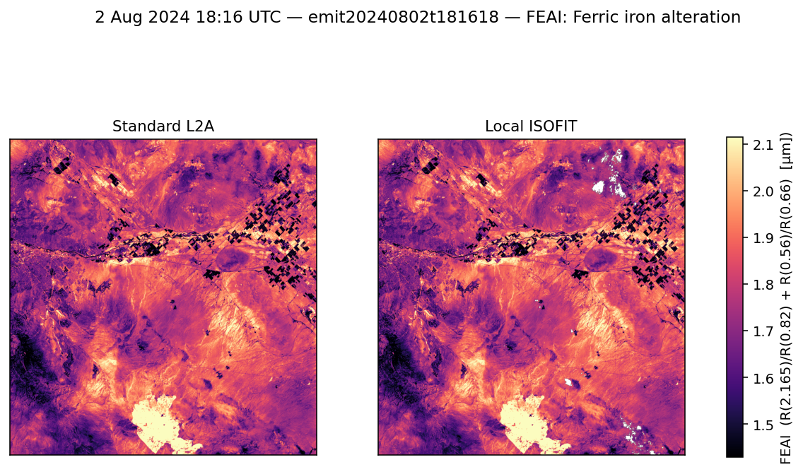
Mineral spectral indices for 2 Aug 2024 18:16 UTC — emit20240802t181618 (15 maps)
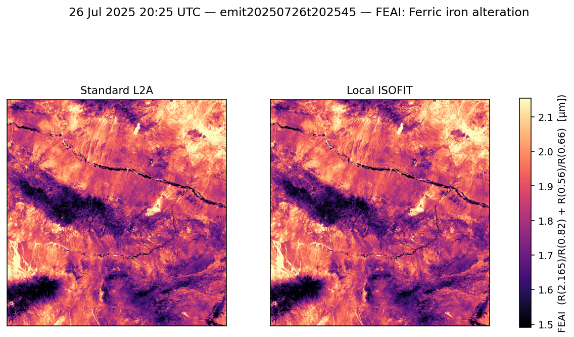
FEAI — Ferric iron alteration
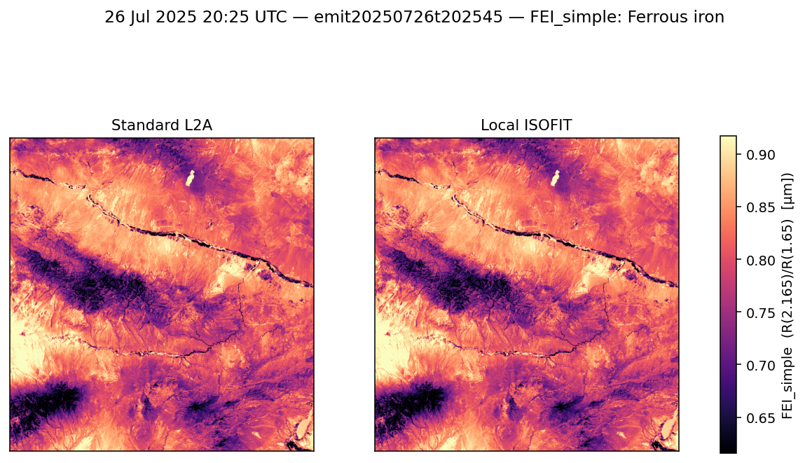
FEI_simple — Ferrous iron
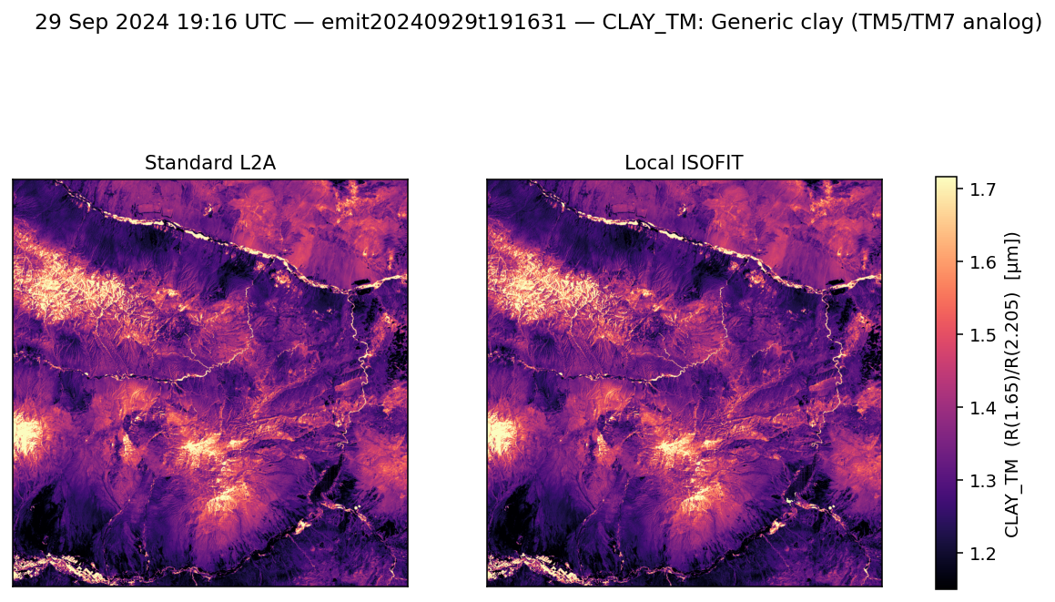
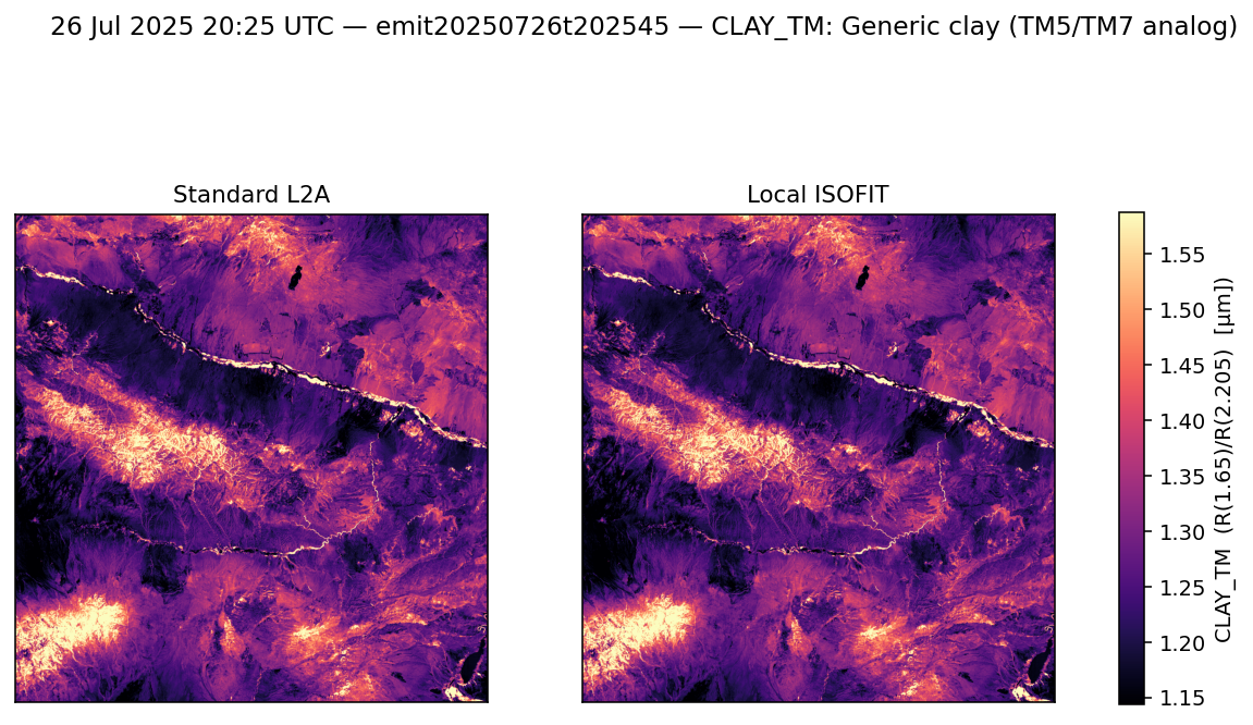
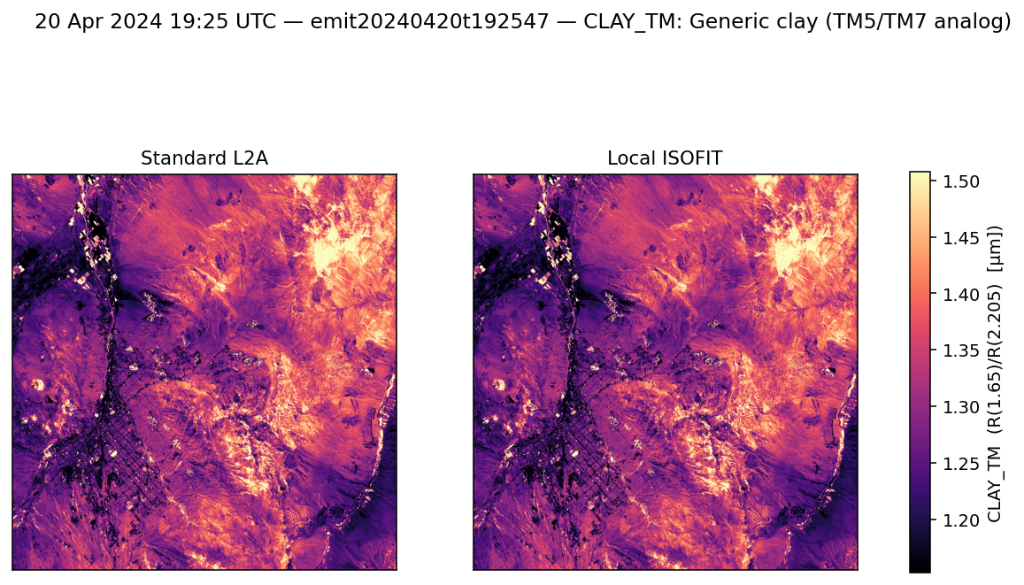
CLAY_TM — Generic clay (TM5/TM7 analog)
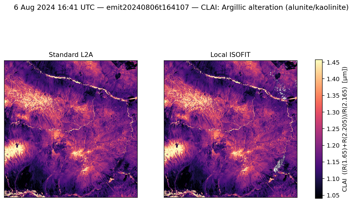
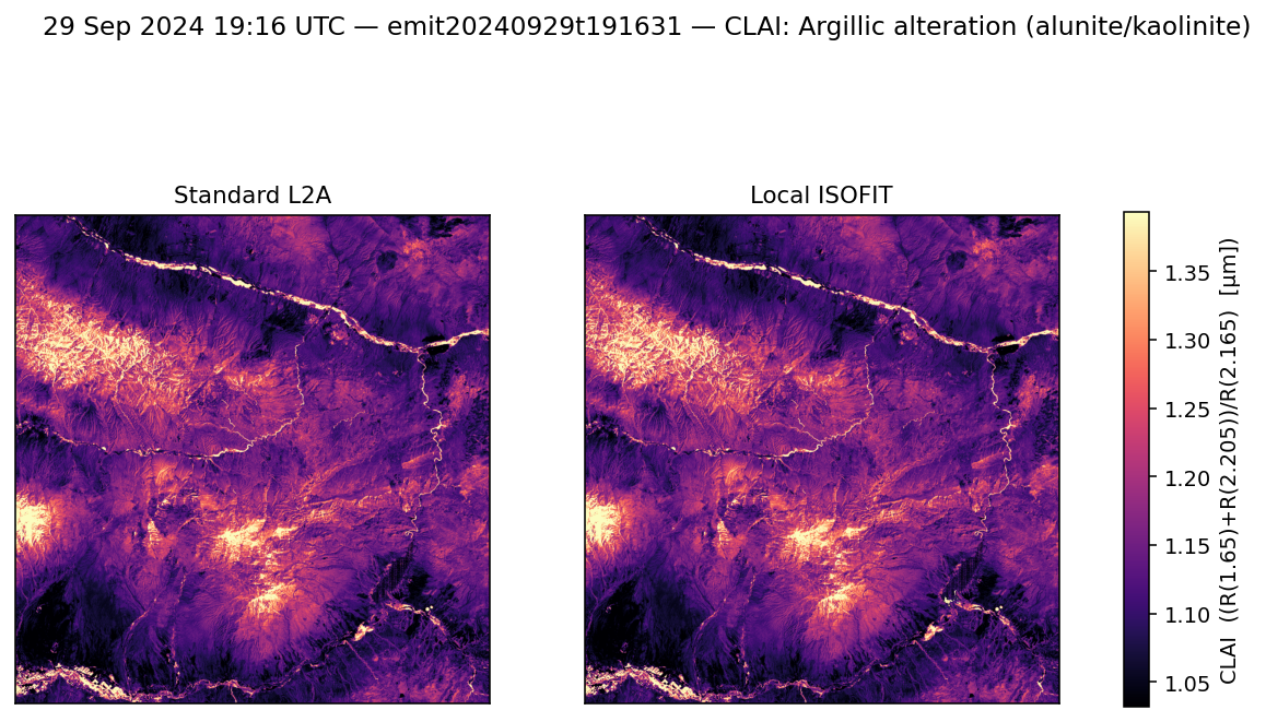
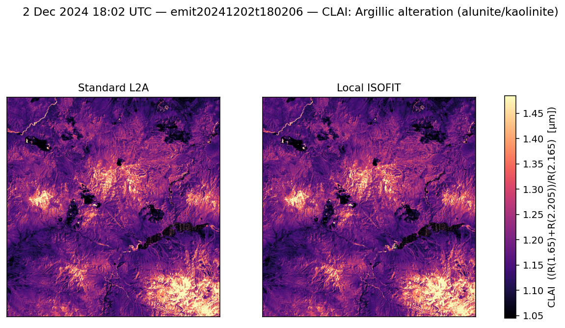
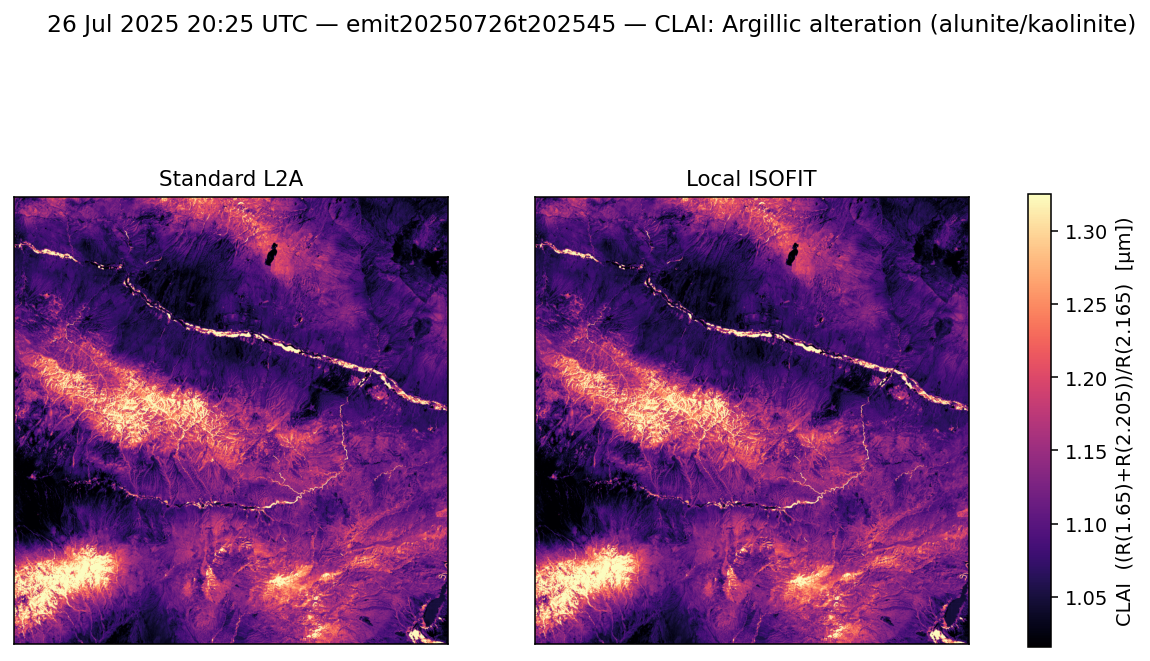
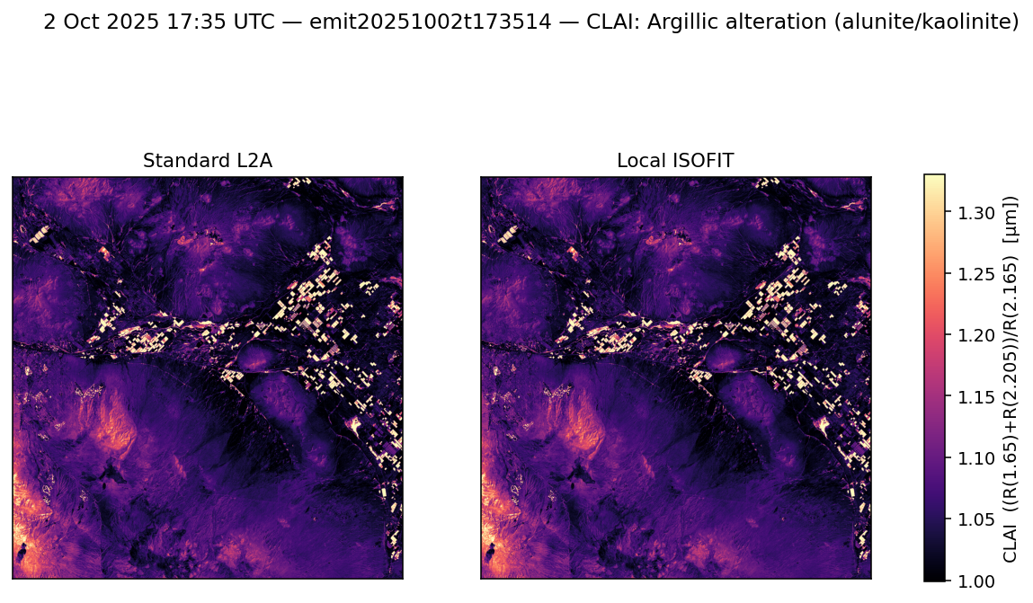
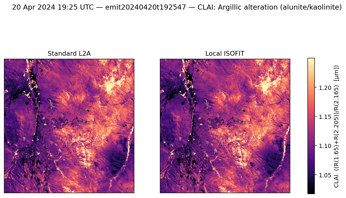
CLAI — Argillic alteration (alunite/kaolinite)
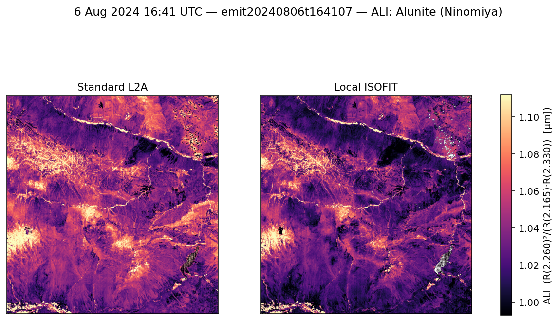
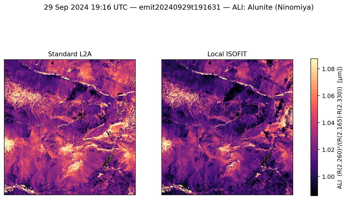
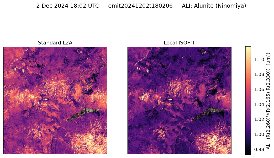
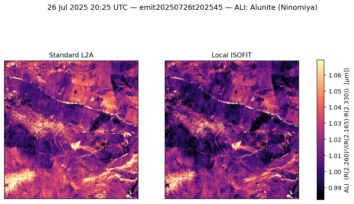
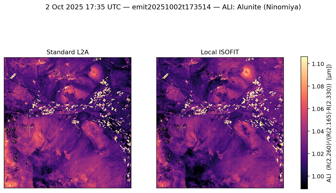
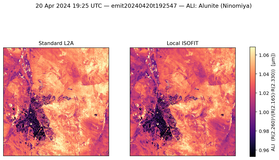
ALI — Alunite (Ninomiya)
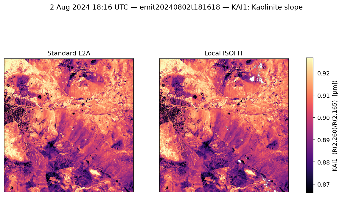
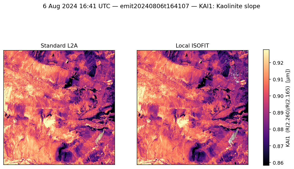
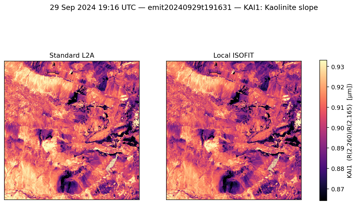
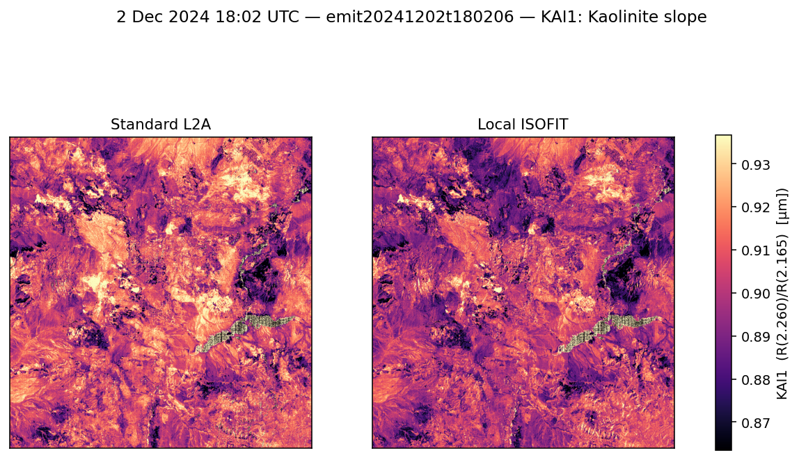
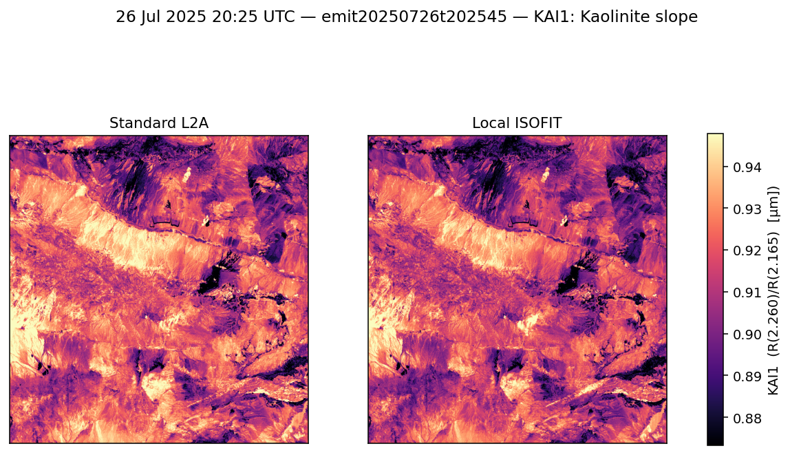
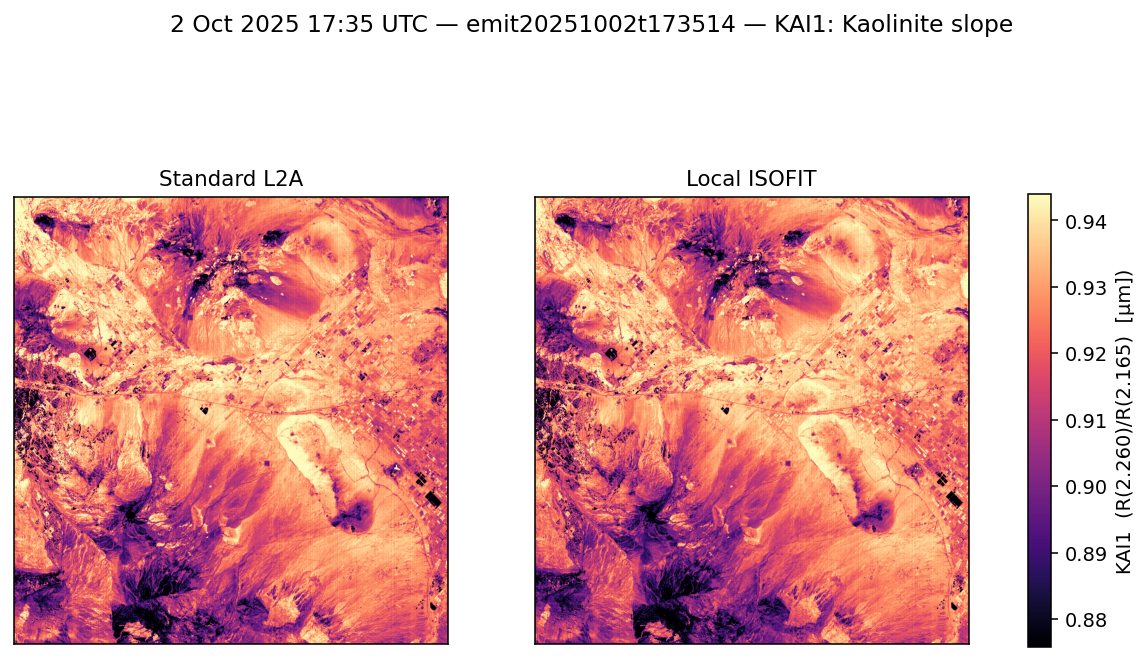
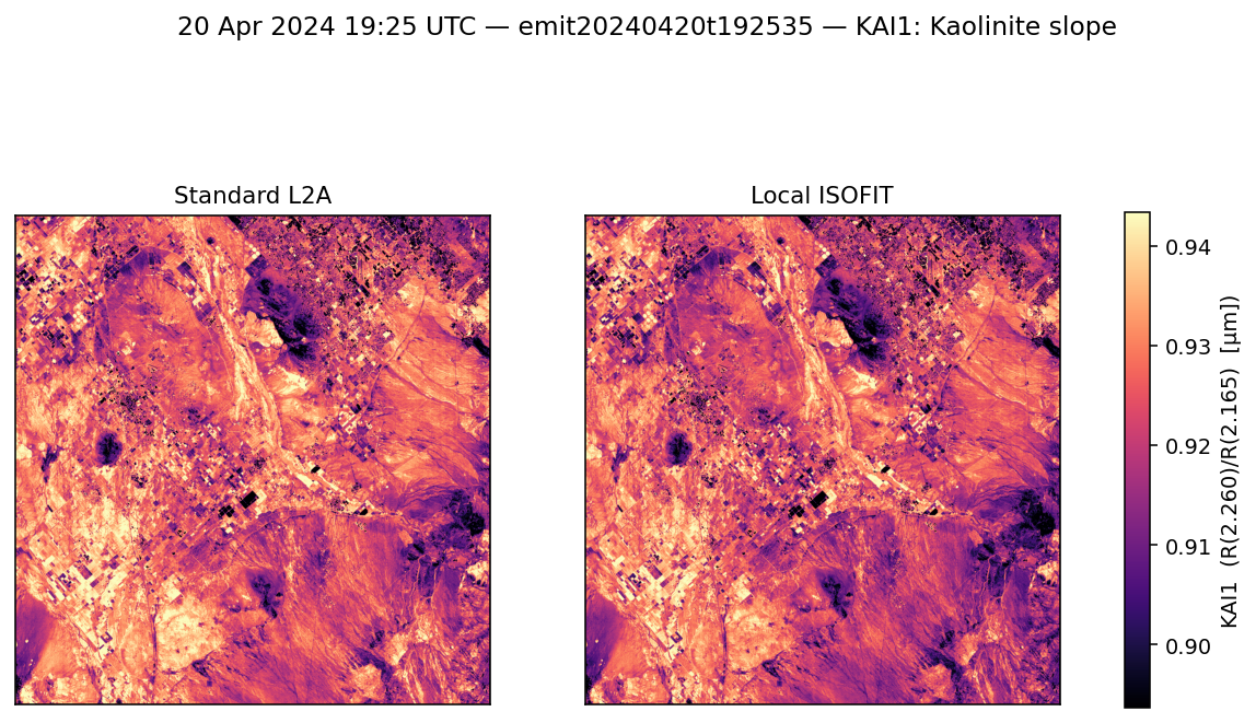
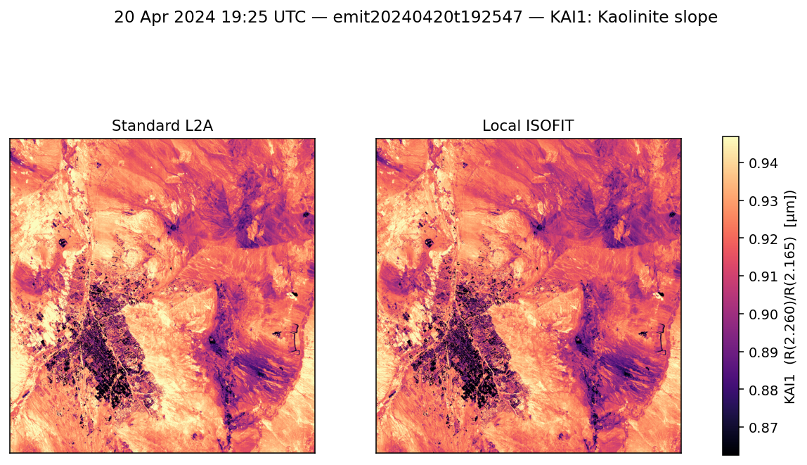
KAI1 — Kaolinite slope
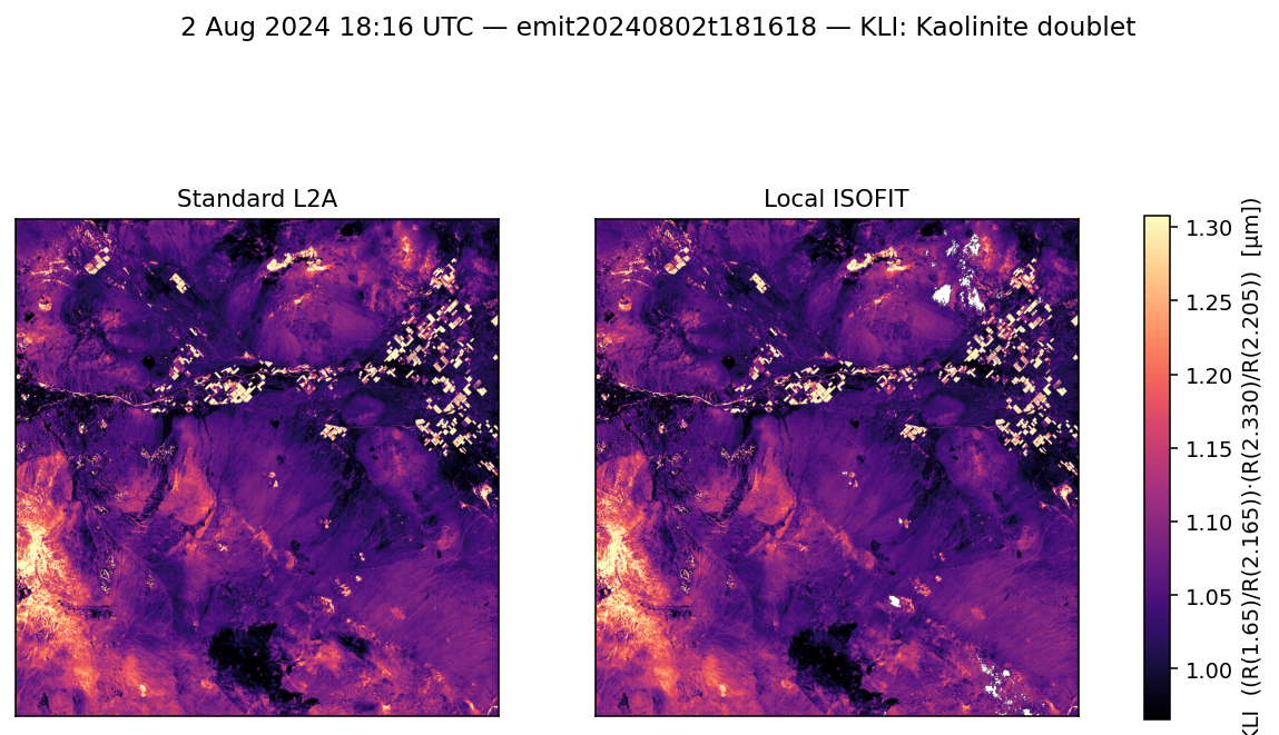
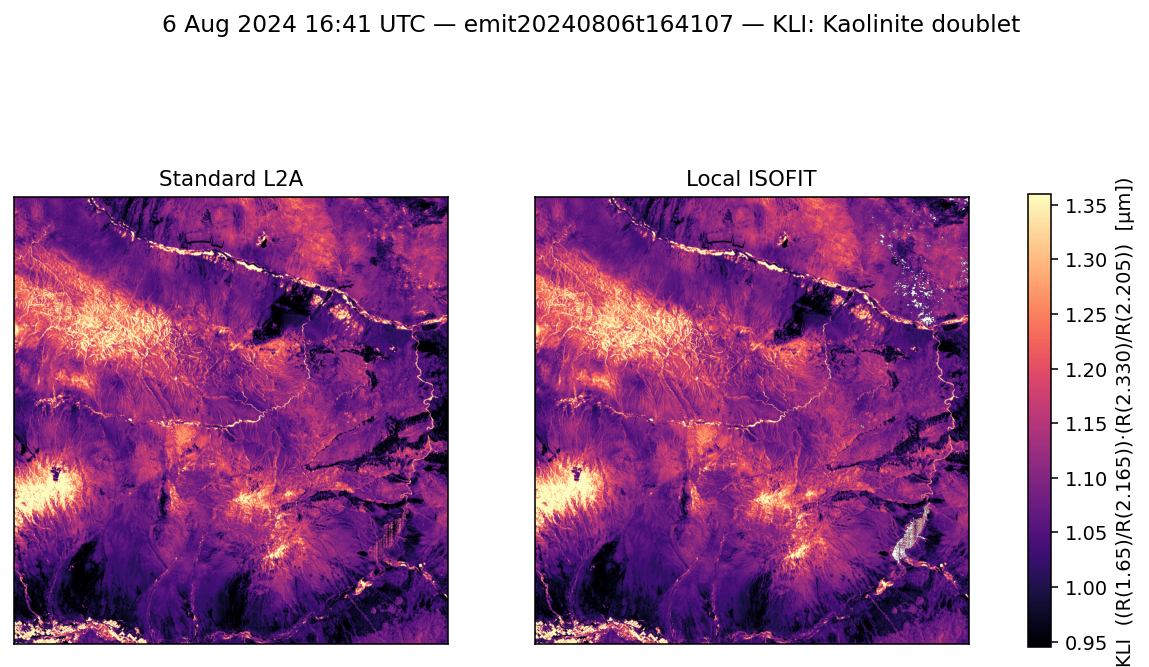
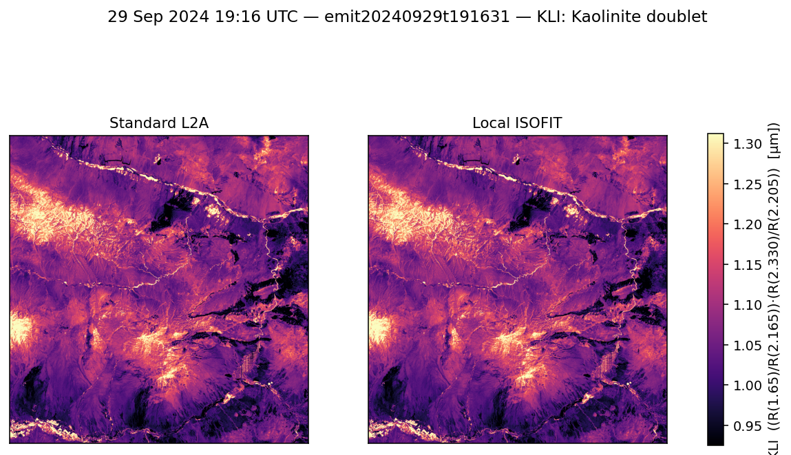
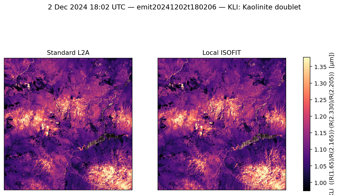
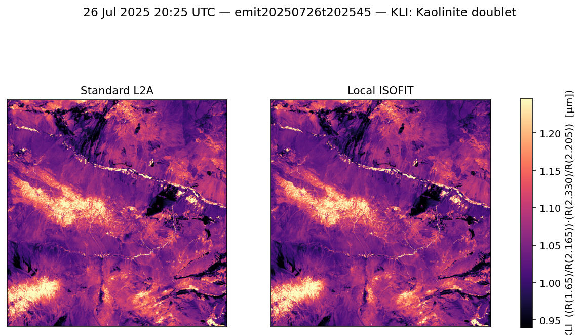
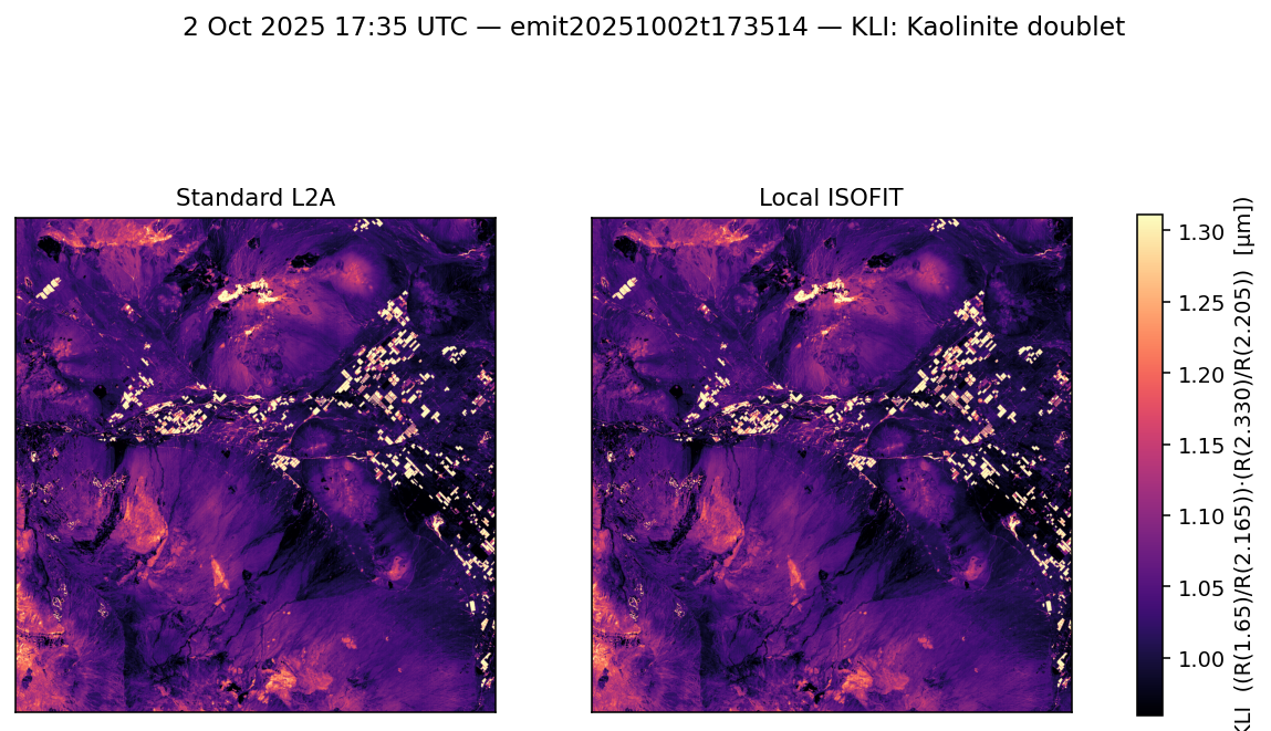
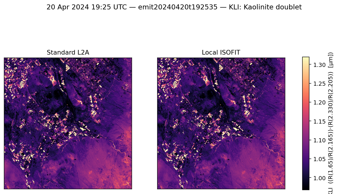
KLI — Kaolinite doublet
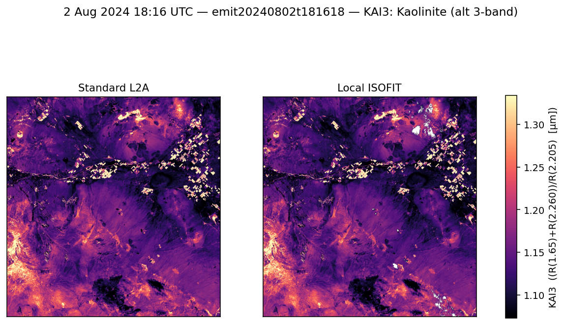
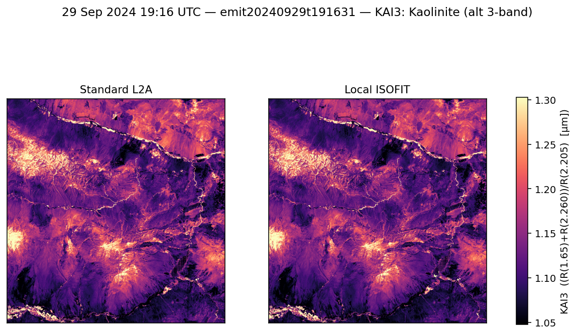
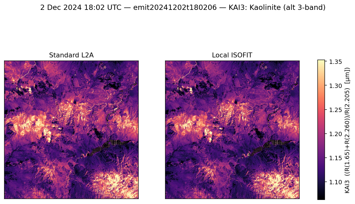
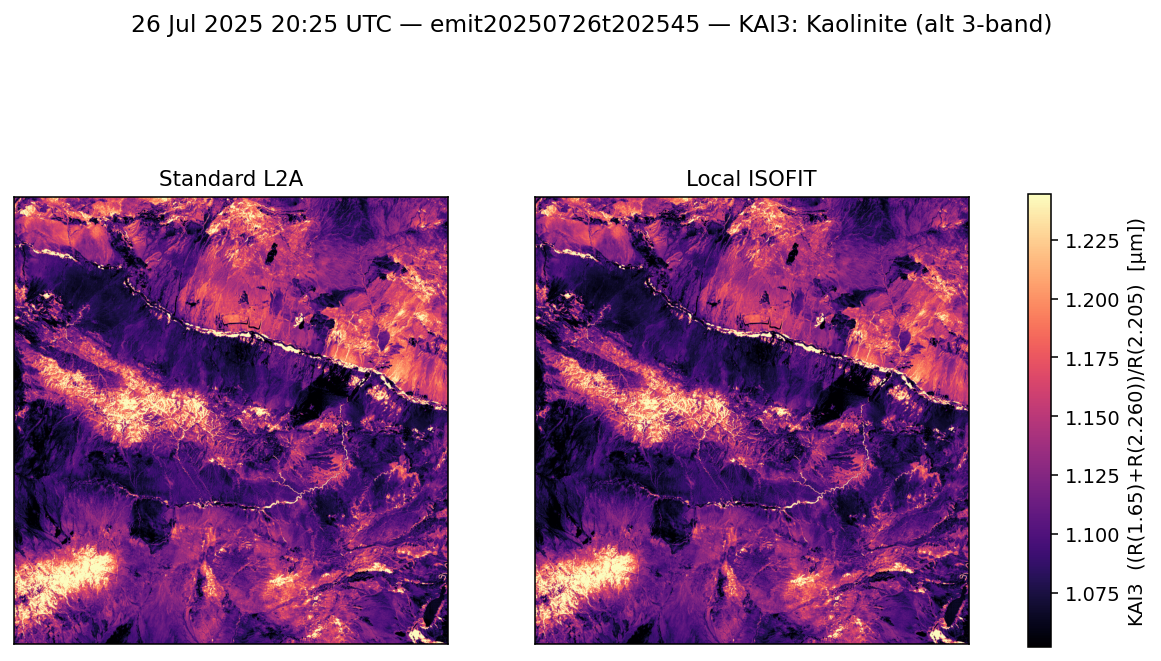
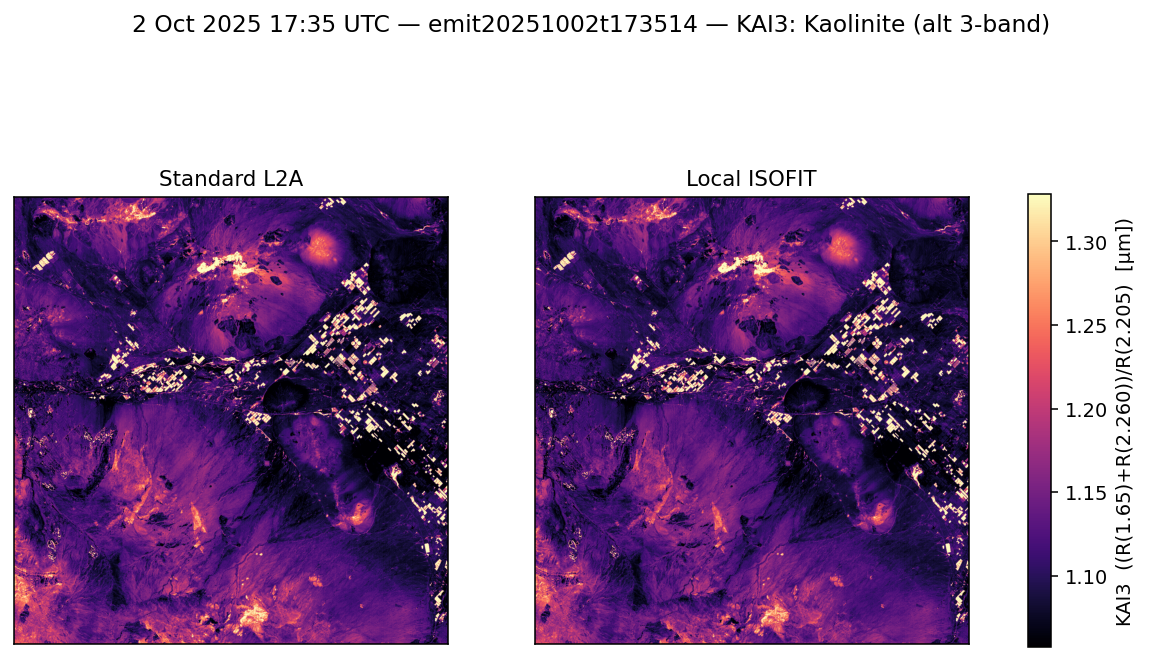
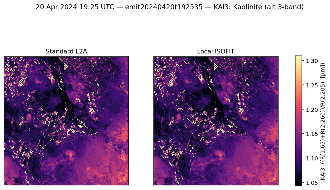
KAI3 — Kaolinite (alt 3-band)
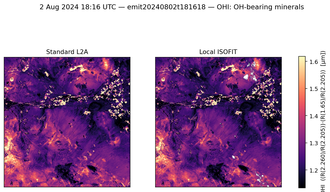
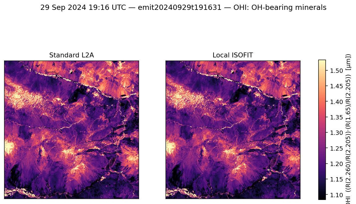
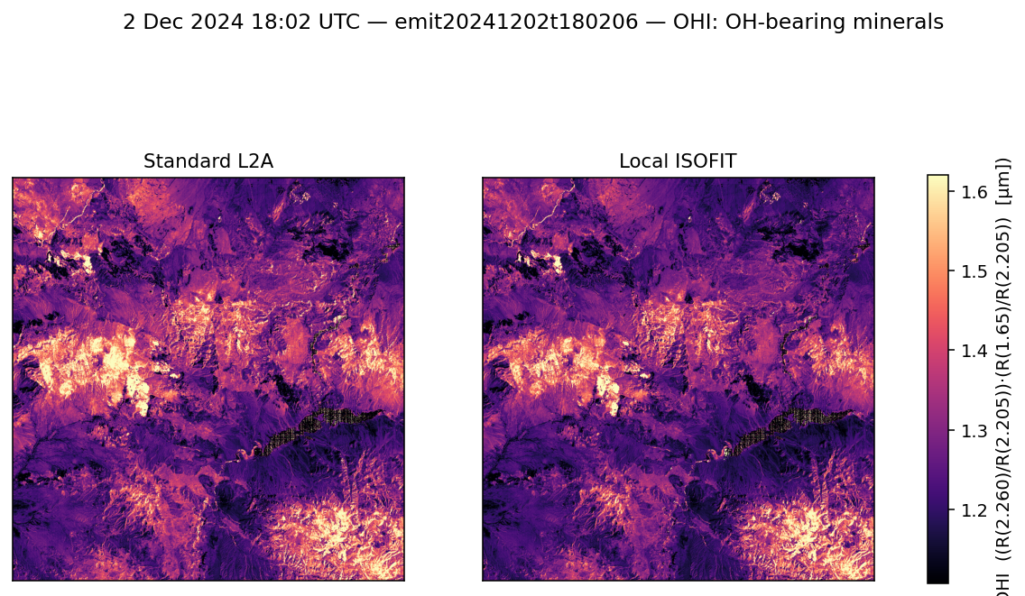
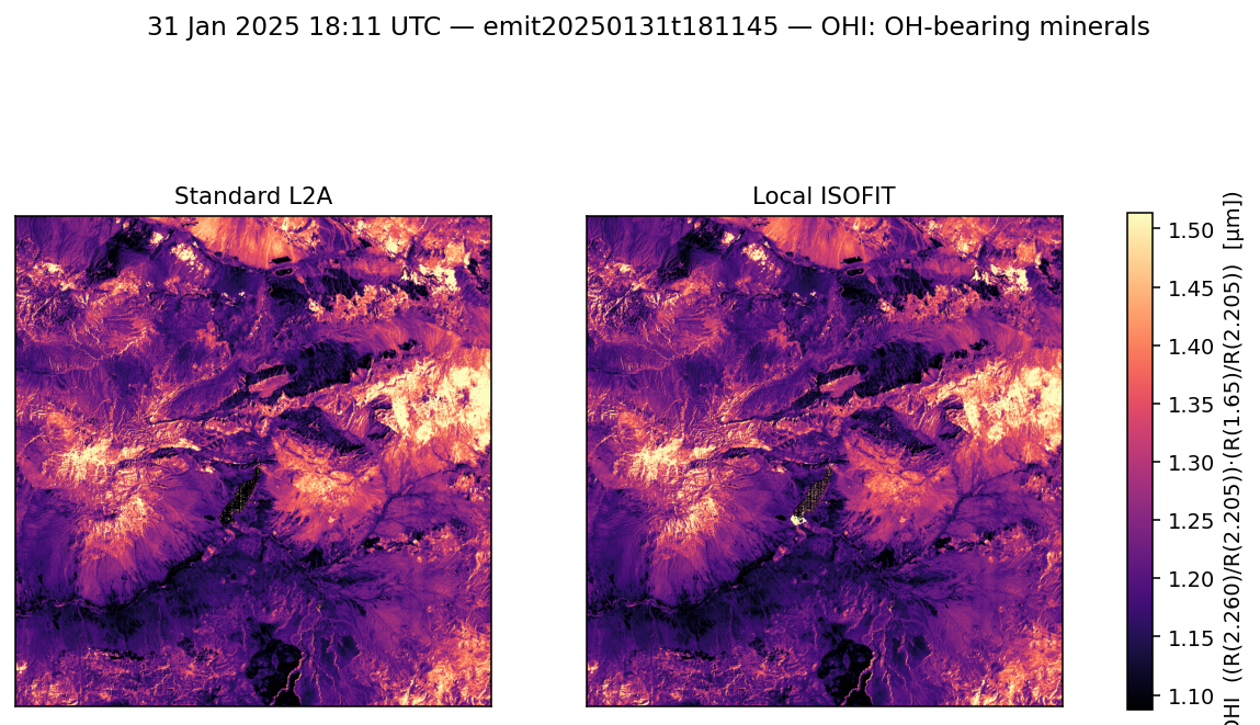
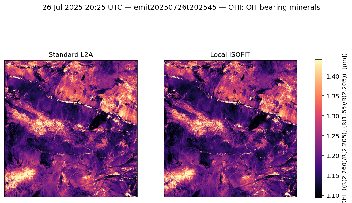
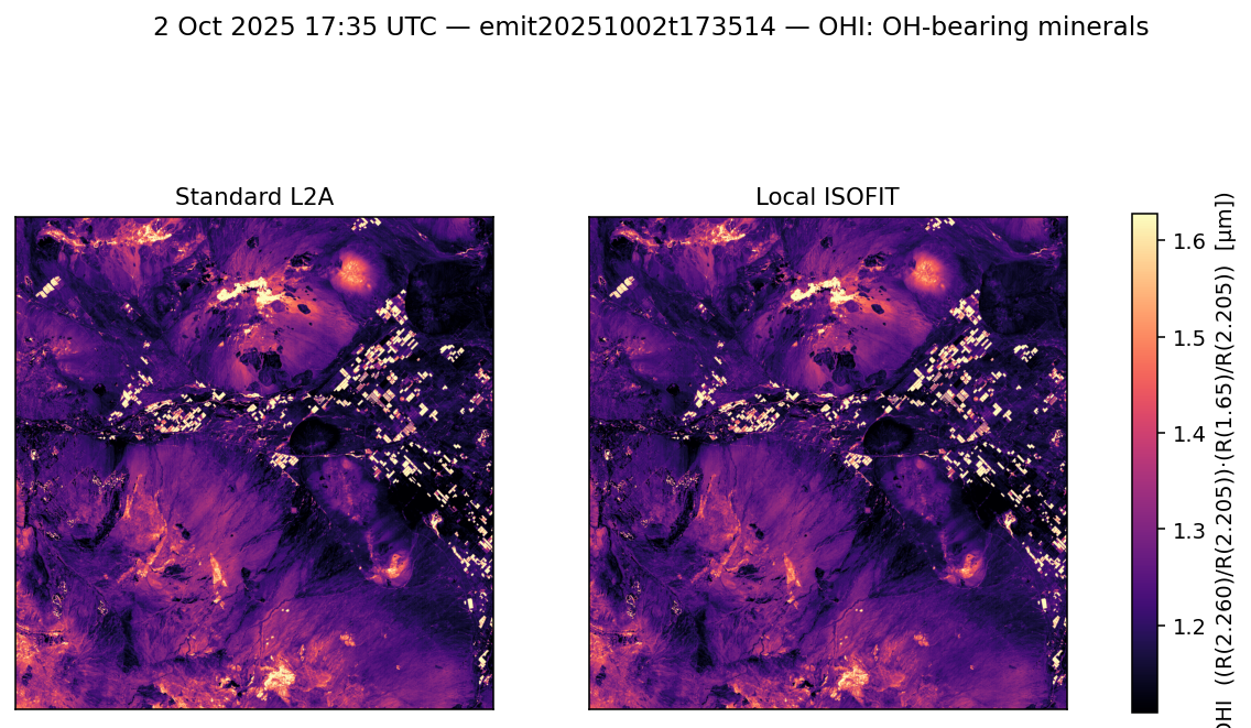
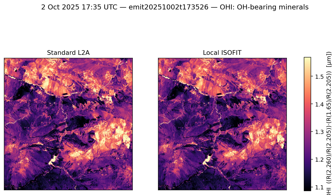
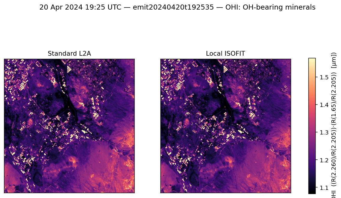
OHI — OH-bearing minerals
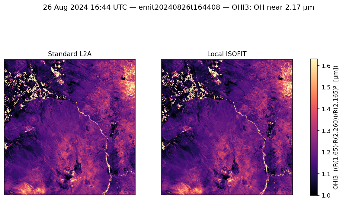
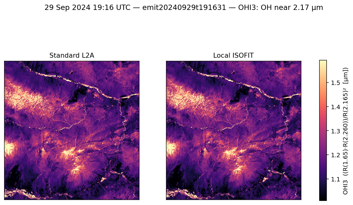
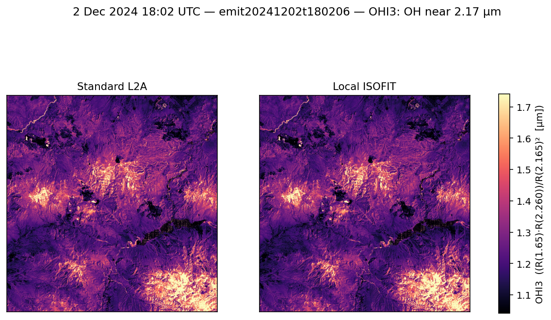
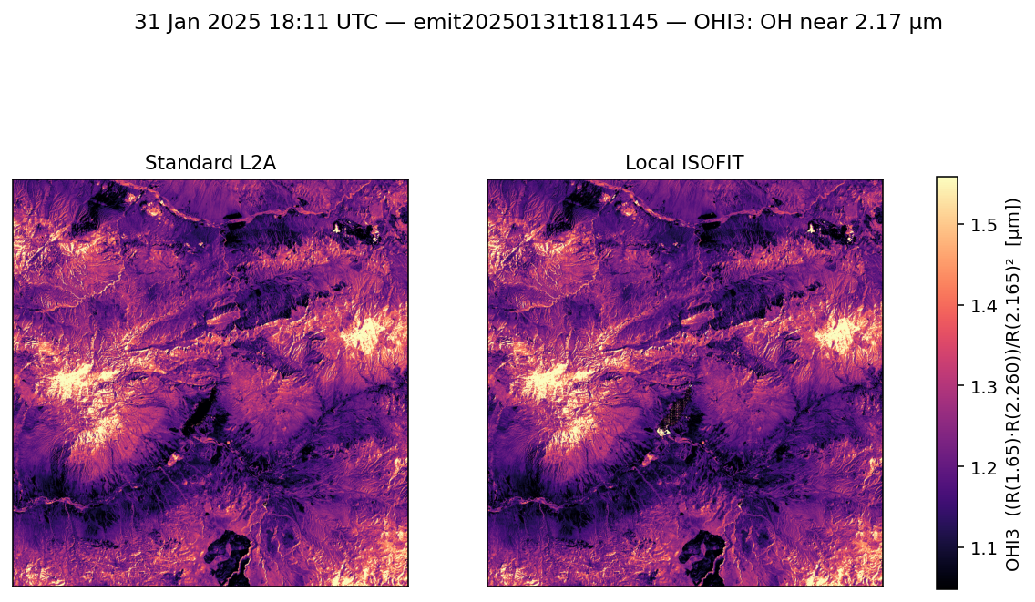
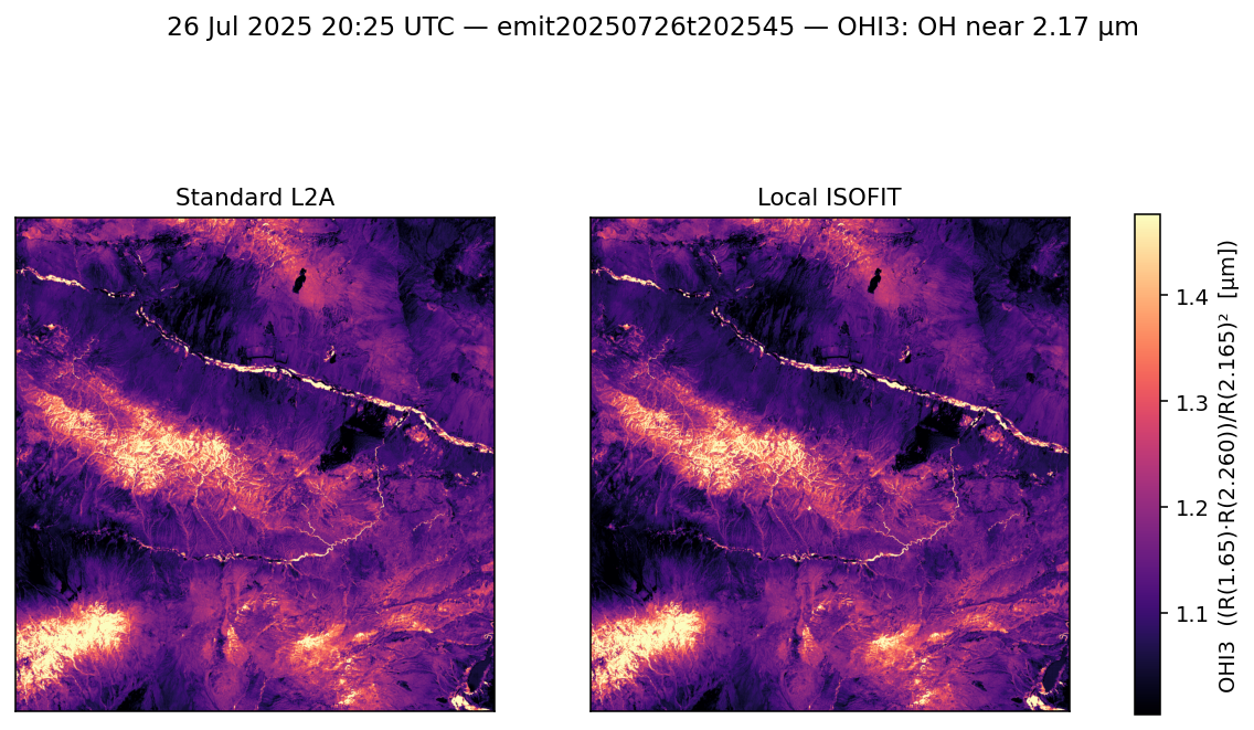
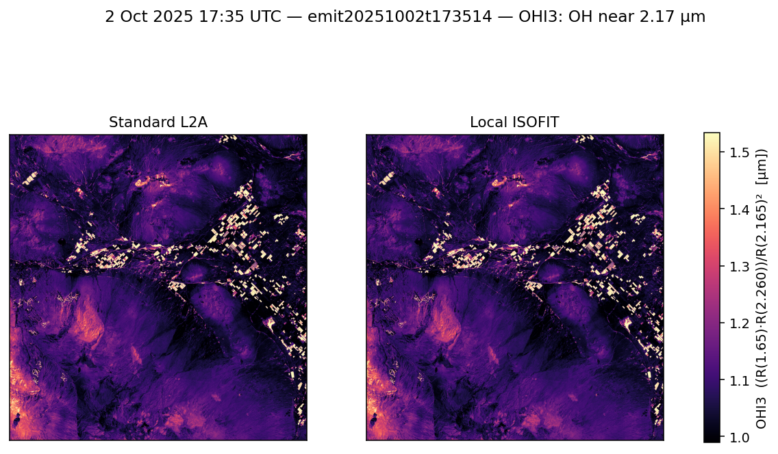
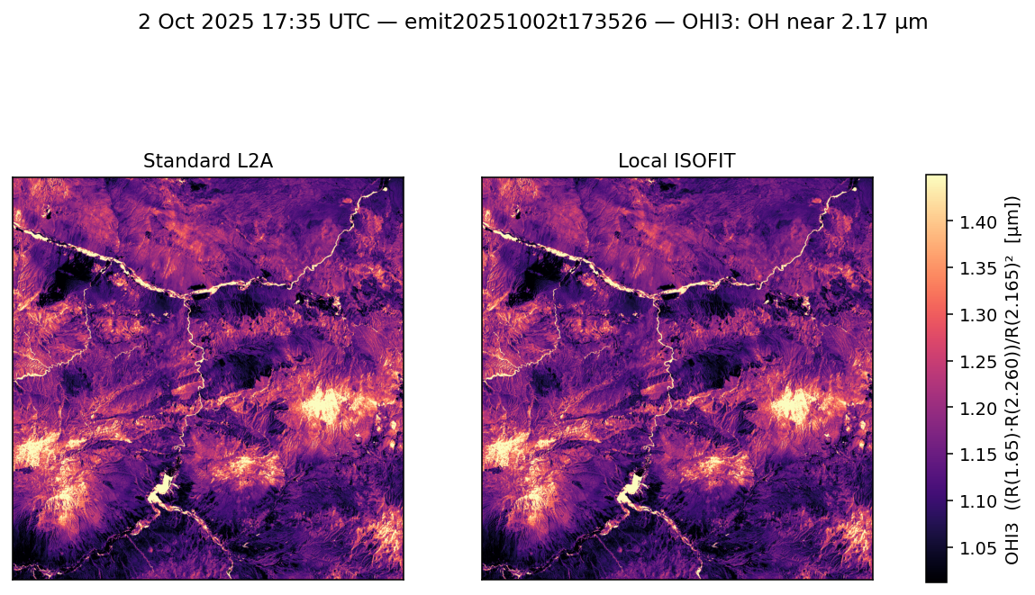
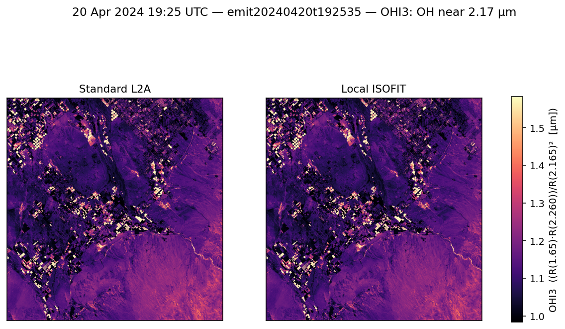
OHI3 — OH near 2.17 µm

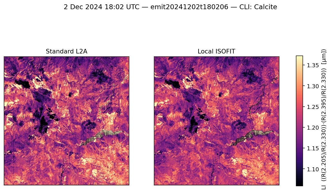
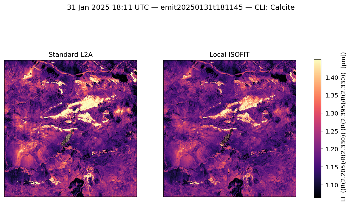
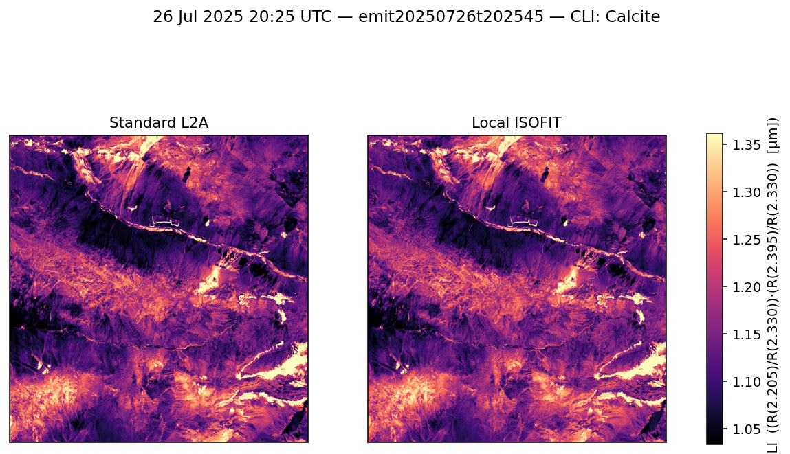
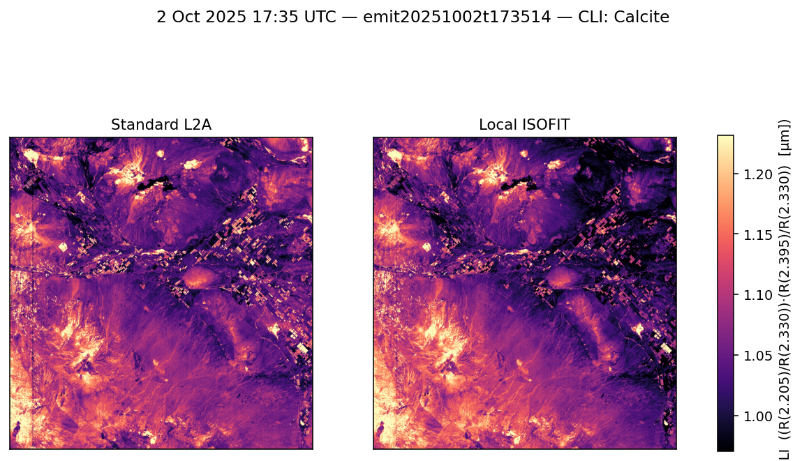
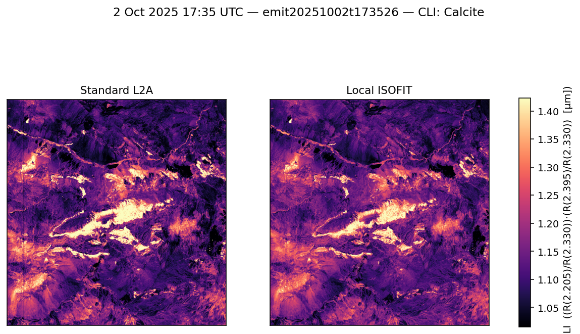
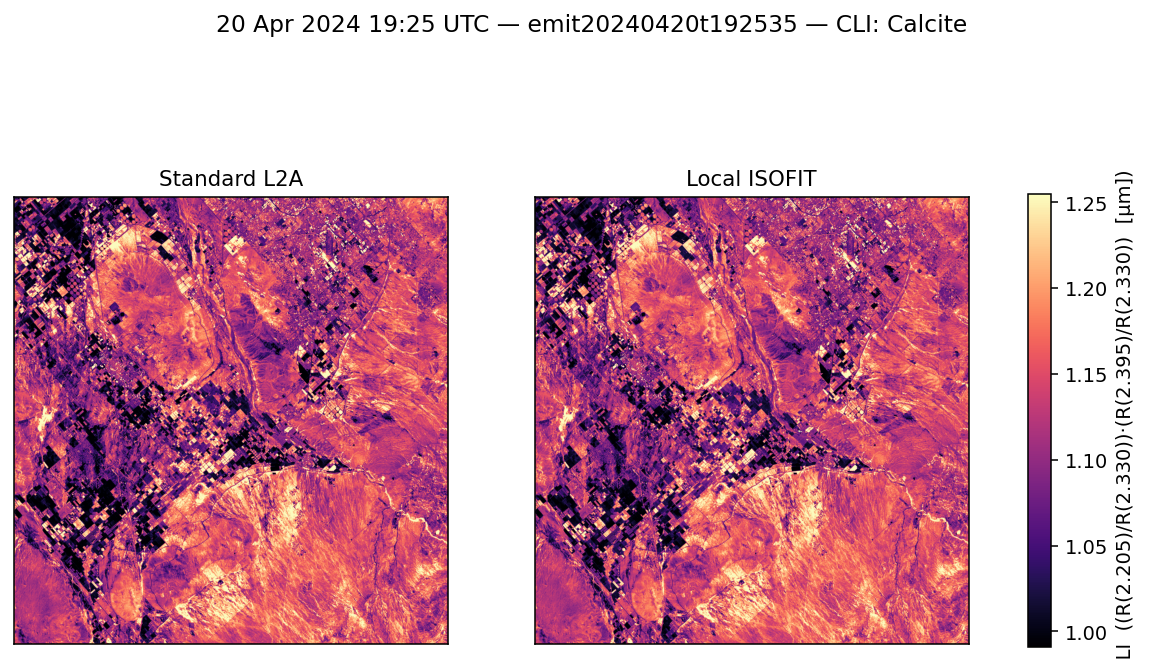
CLI — Calcite
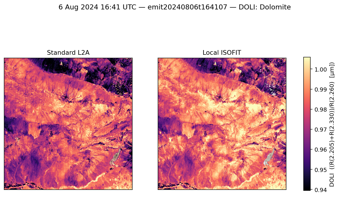
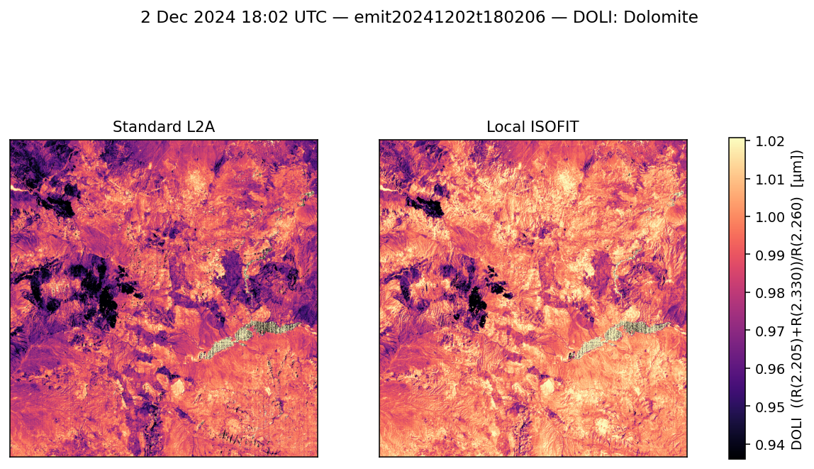
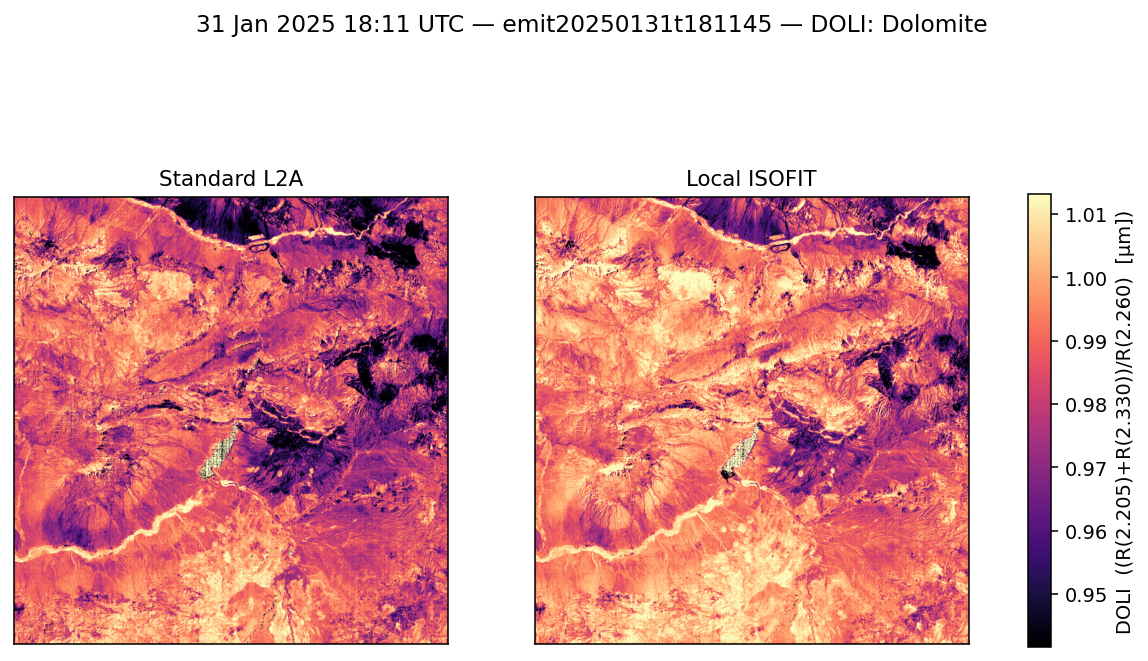
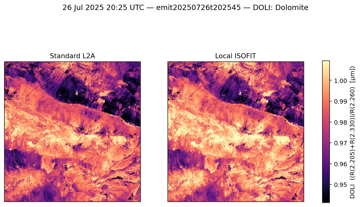
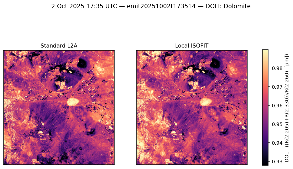
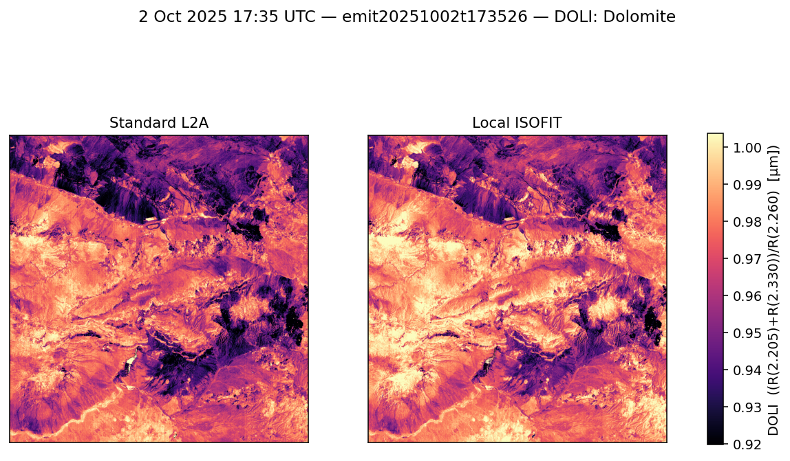
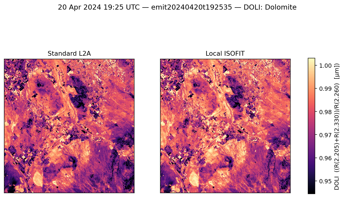
DOLI — Dolomite
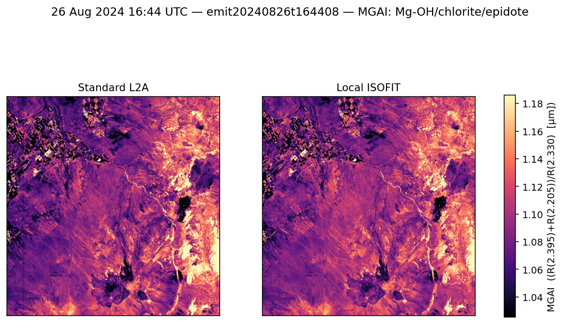
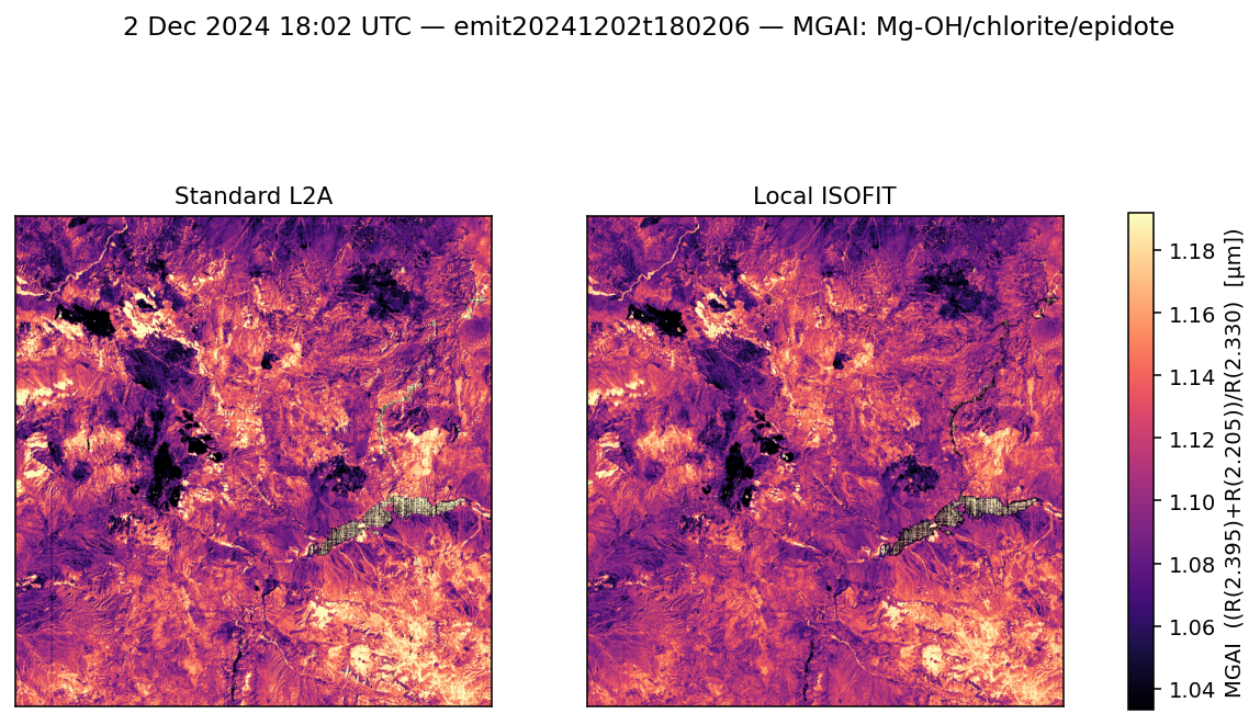
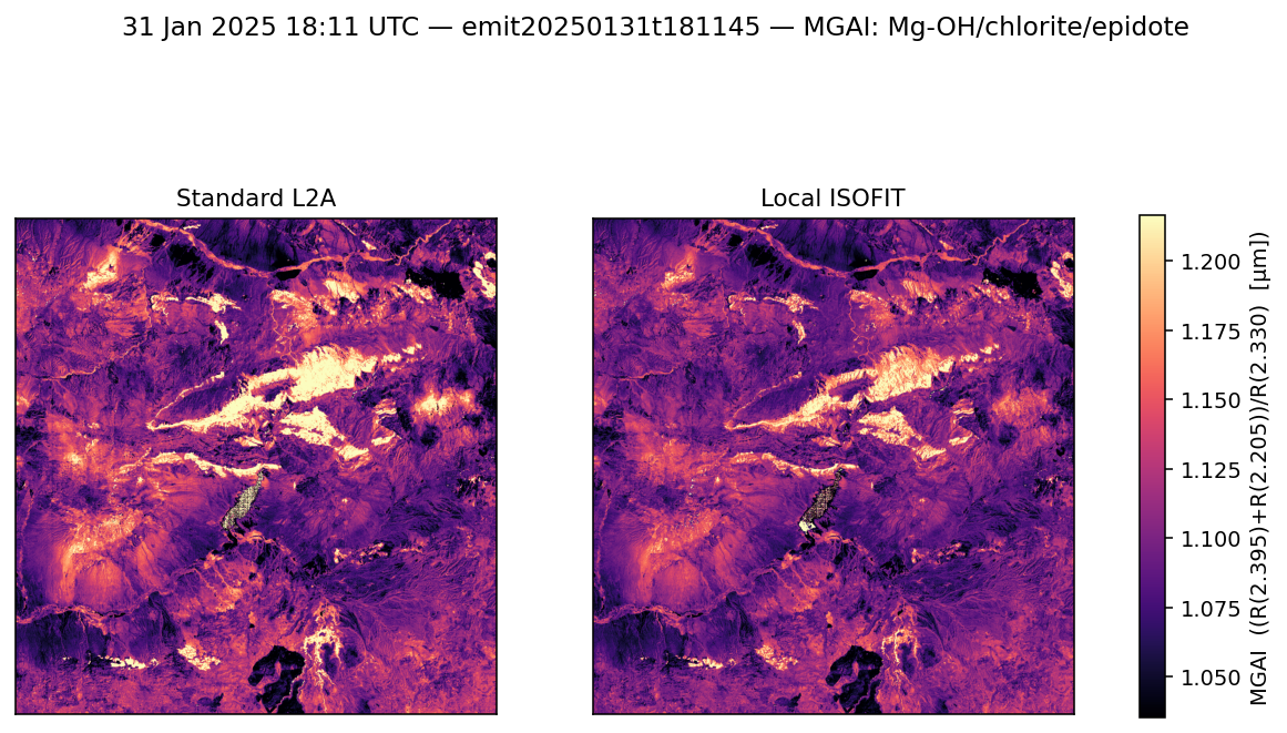
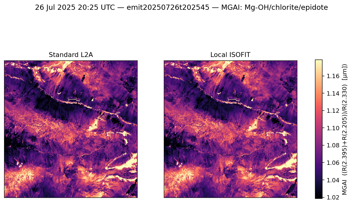
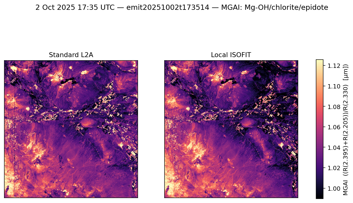
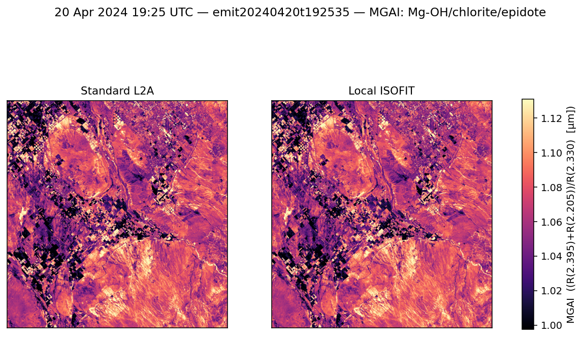
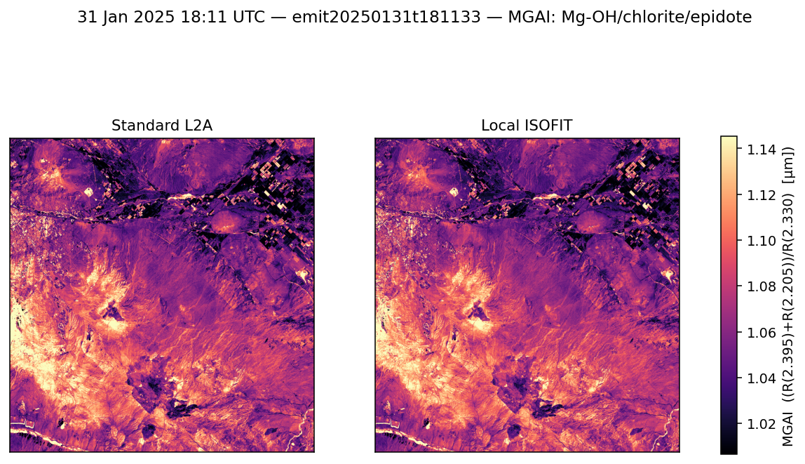
MGAI — Mg-OH/chlorite/epidote
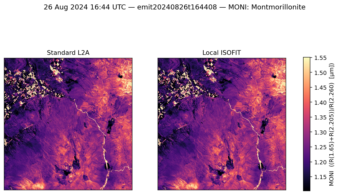
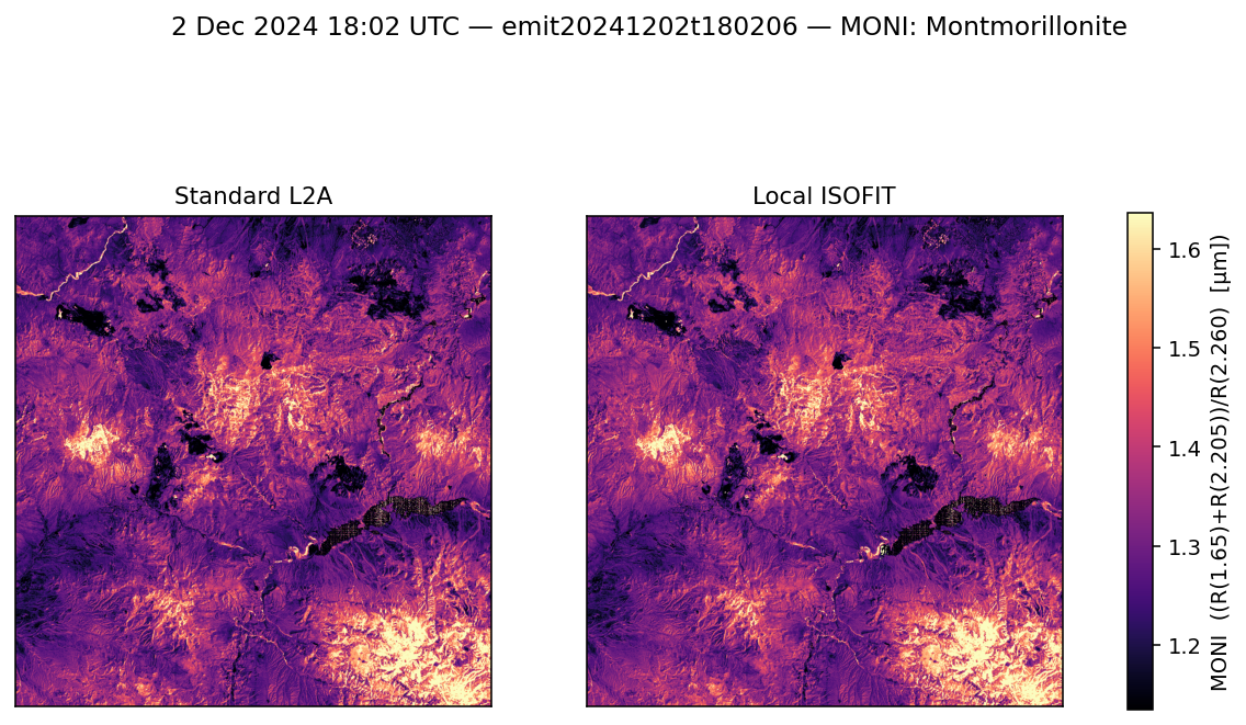
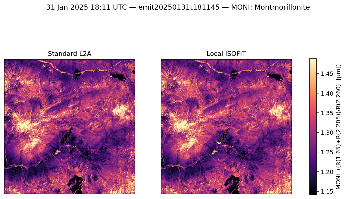
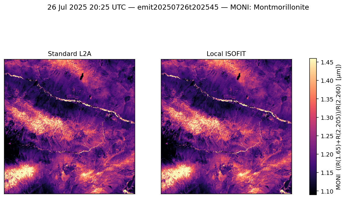
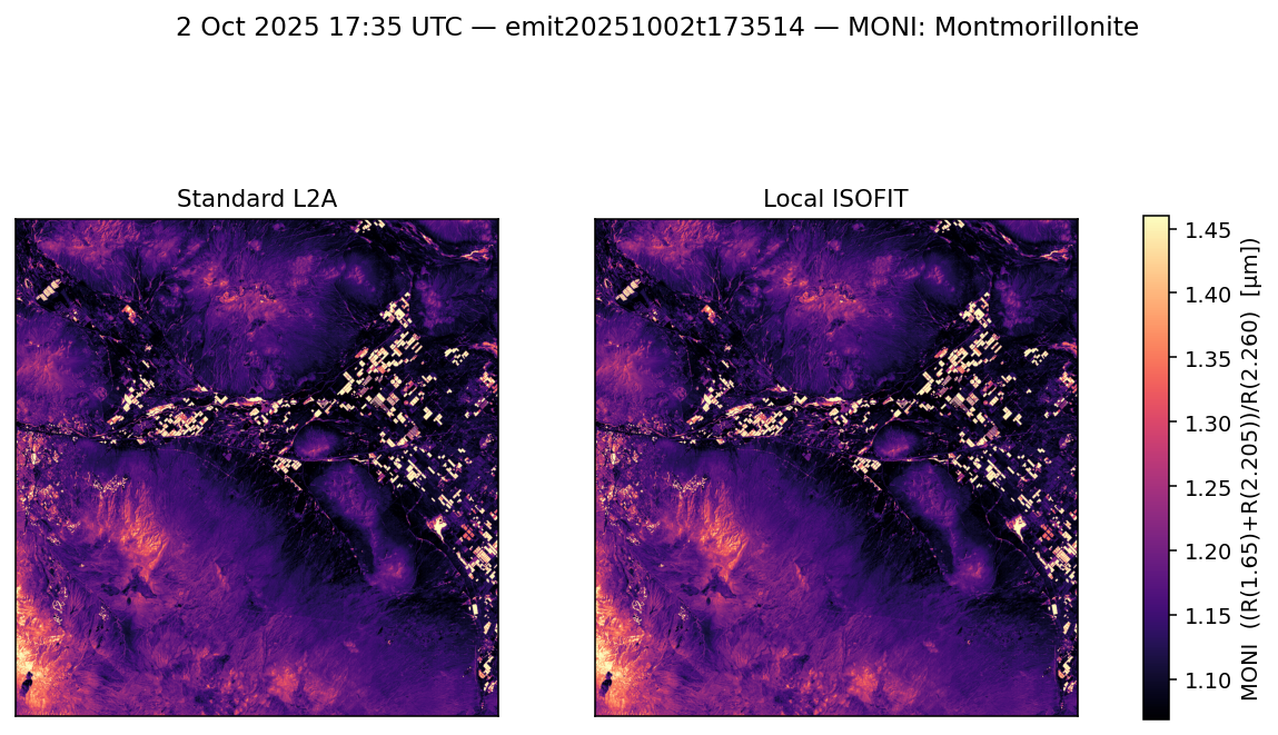
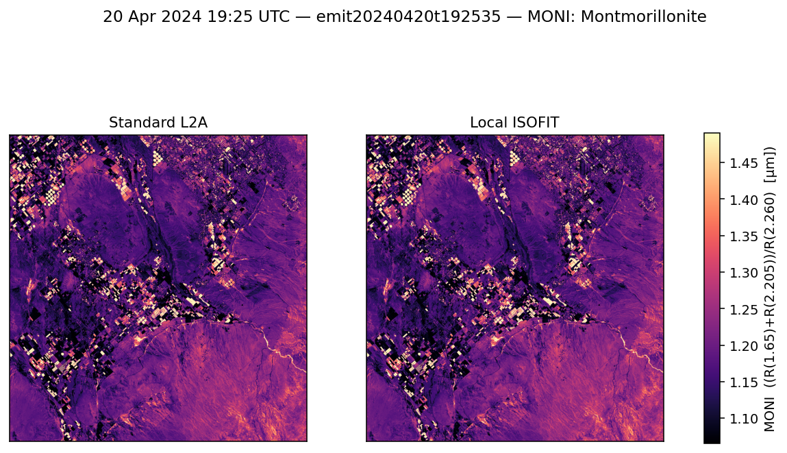
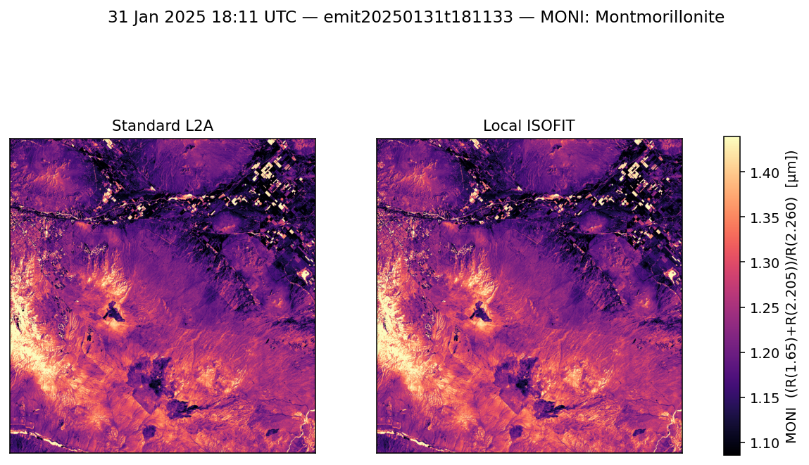
MONI — Montmorillonite
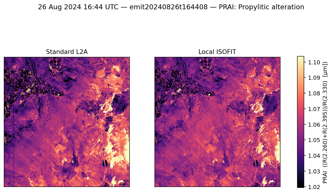
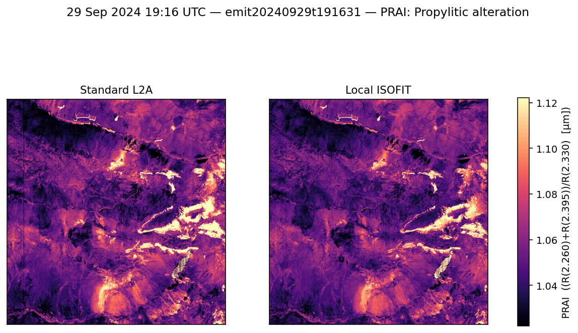
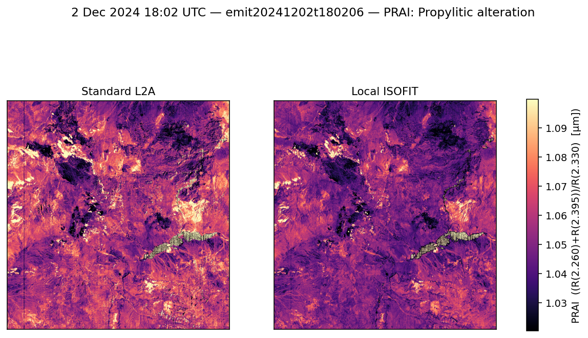
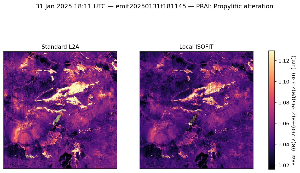
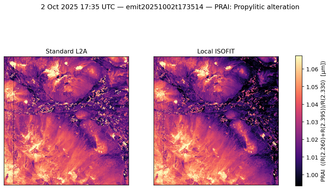
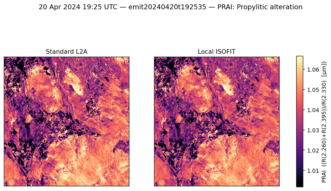
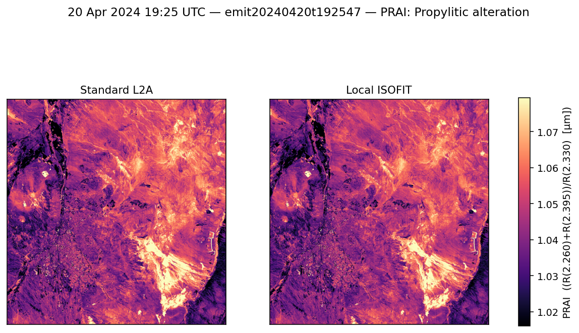
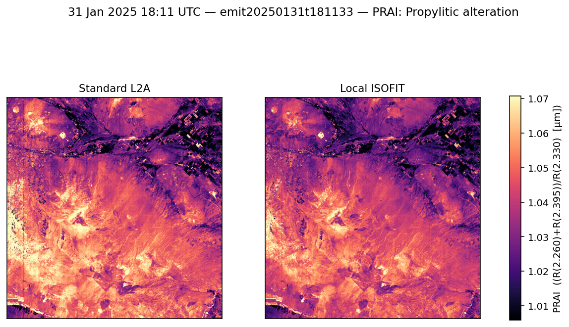
PRAI — Propylitic alteration
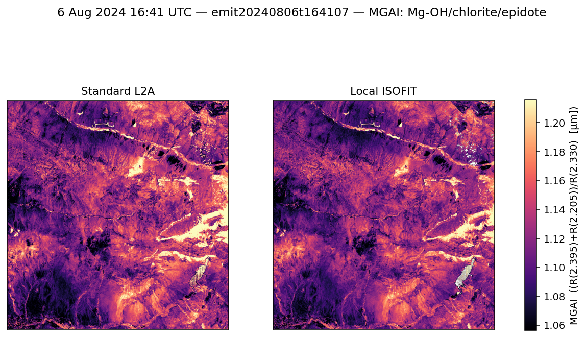
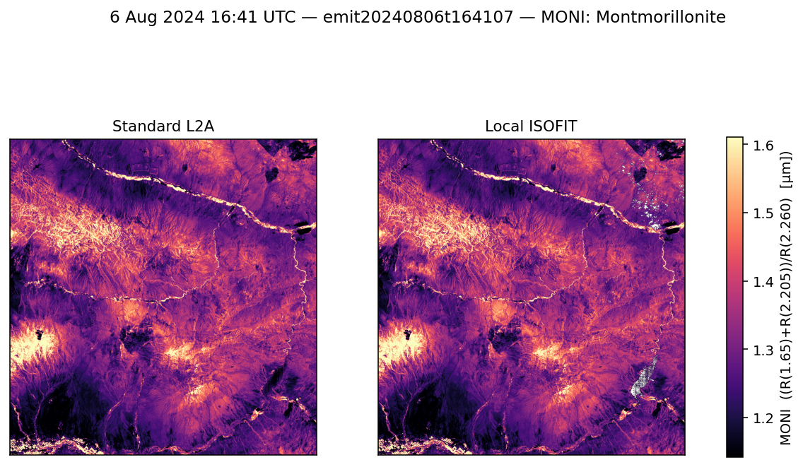
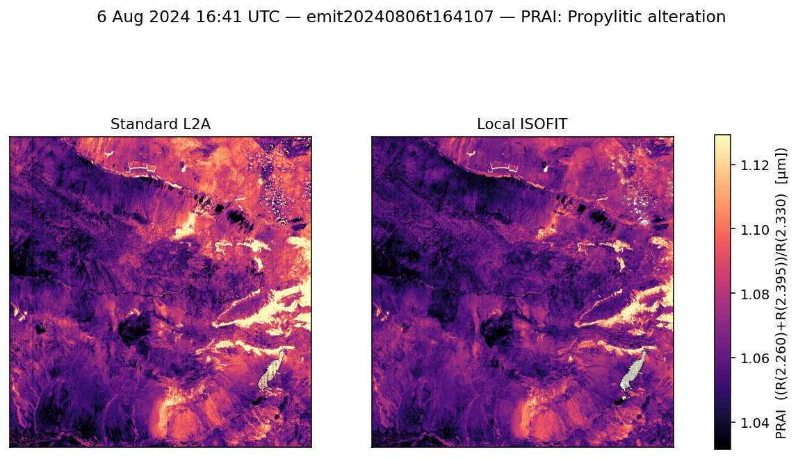
6 Aug 2024 16:41 UTC — emit20240806t164107
Click to expand spectra, PCA grid, eigenvalues, and mineral indices
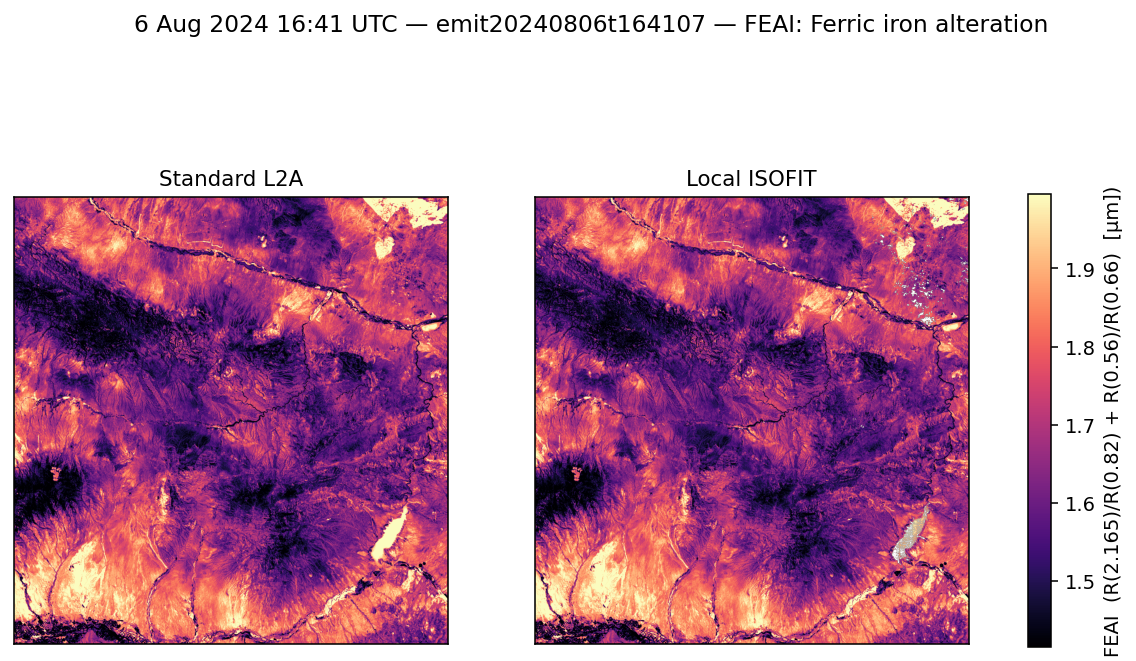
Mineral spectral indices for 6 Aug 2024 16:41 UTC — emit20240806t164107 (15 maps)
FEAI — Ferric iron alteration
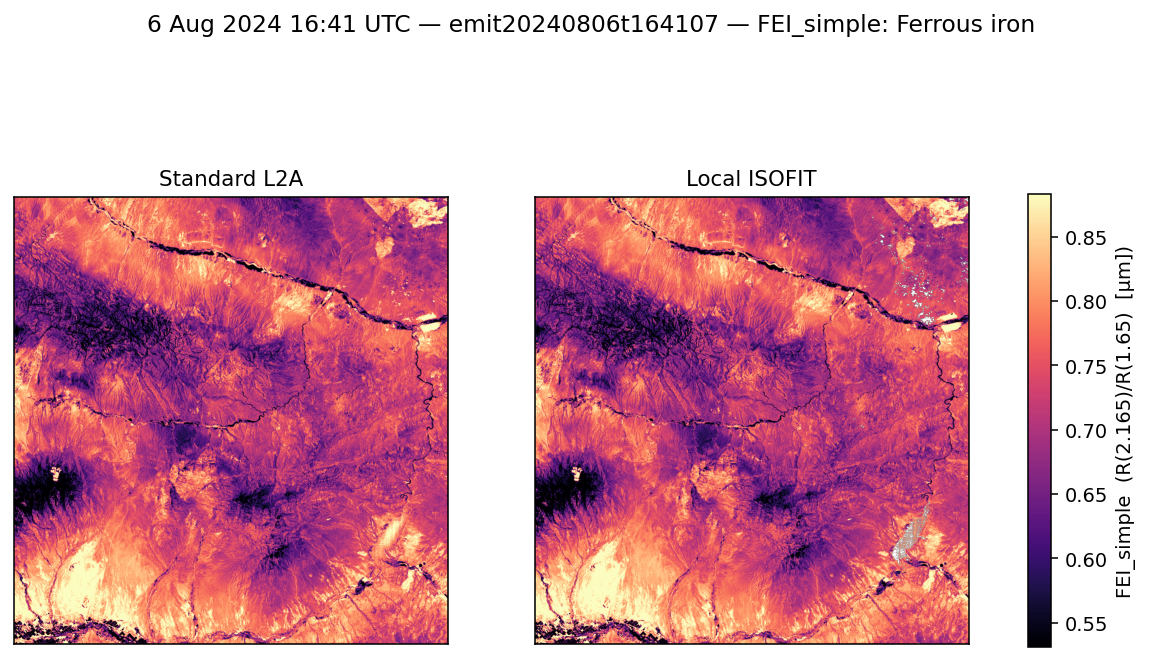
FEI_simple — Ferrous iron
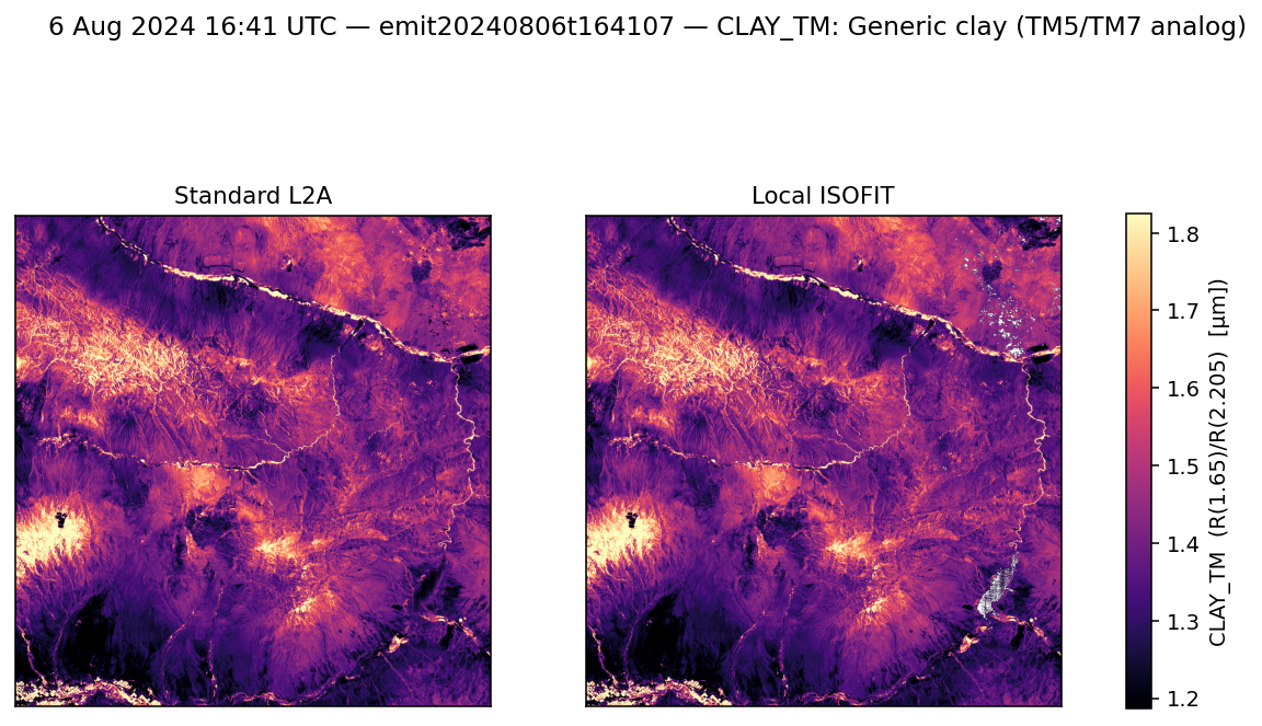
CLAY_TM — Generic clay (TM5/TM7 analog)
CLAI — Argillic alteration (alunite/kaolinite)
ALI — Alunite (Ninomiya)
KAI1 — Kaolinite slope
KLI — Kaolinite doublet
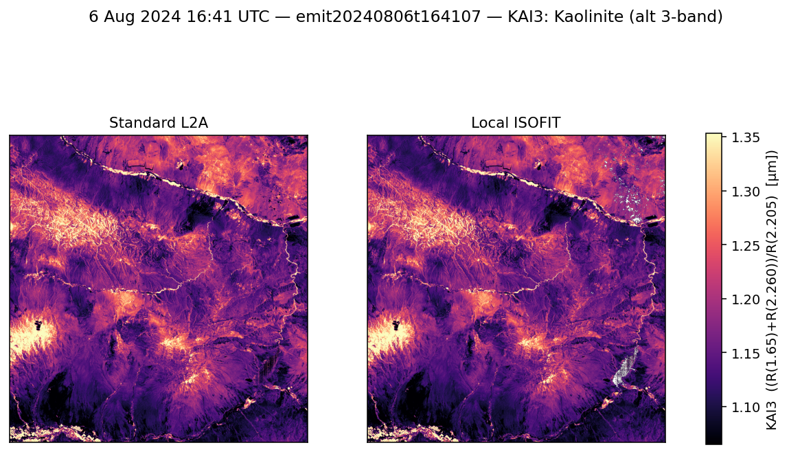
KAI3 — Kaolinite (alt 3-band)
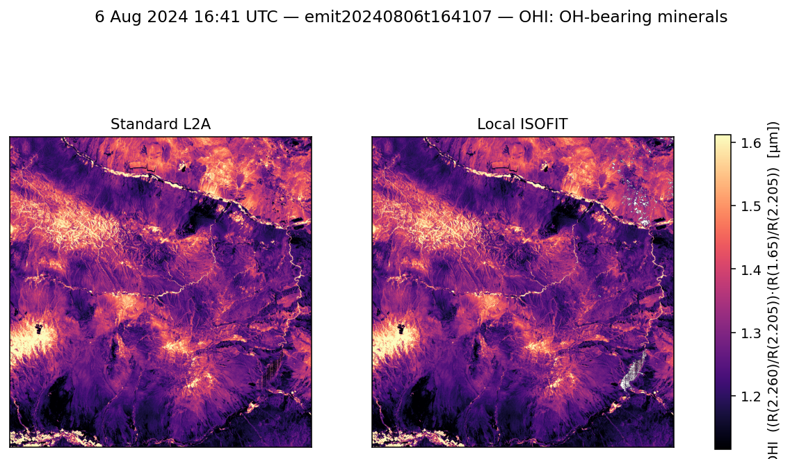
OHI — OH-bearing minerals
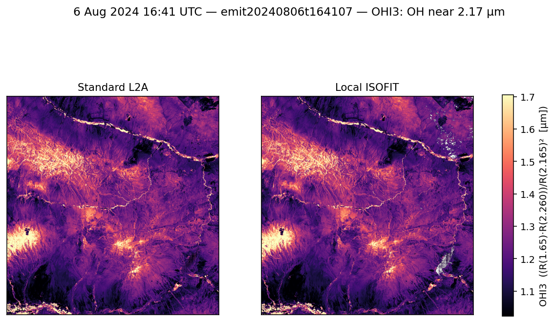
OHI3 — OH near 2.17 µm
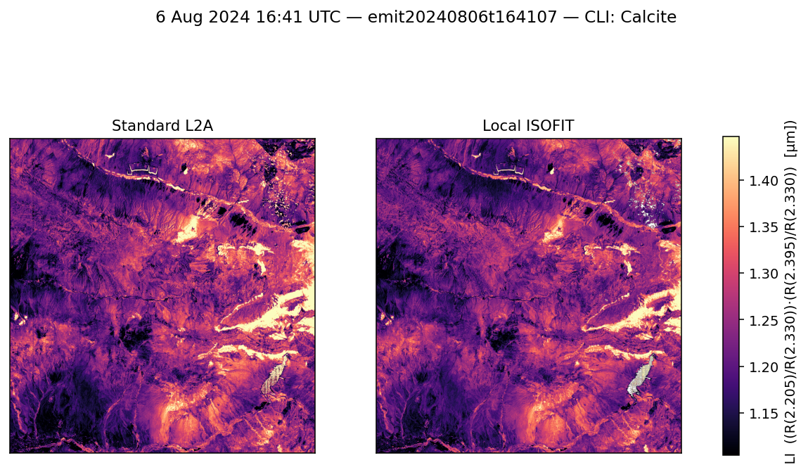
CLI — Calcite
DOLI — Dolomite
MGAI — Mg-OH/chlorite/epidote
MONI — Montmorillonite
PRAI — Propylitic alteration
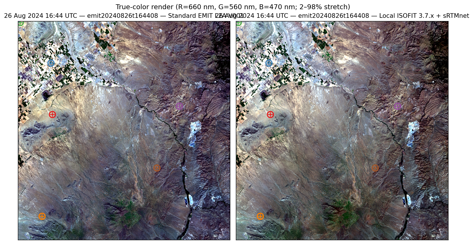
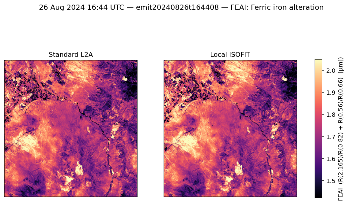
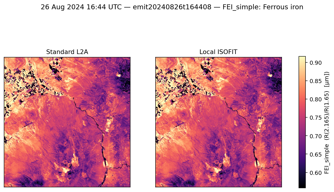
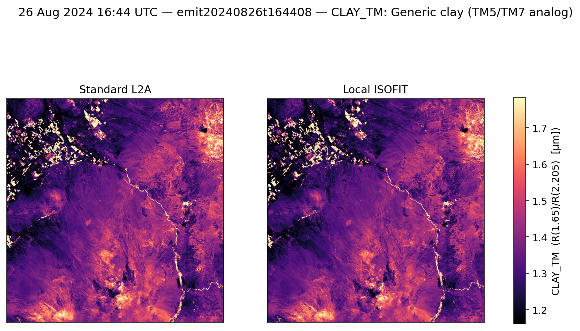
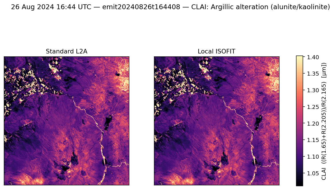
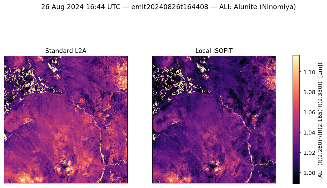
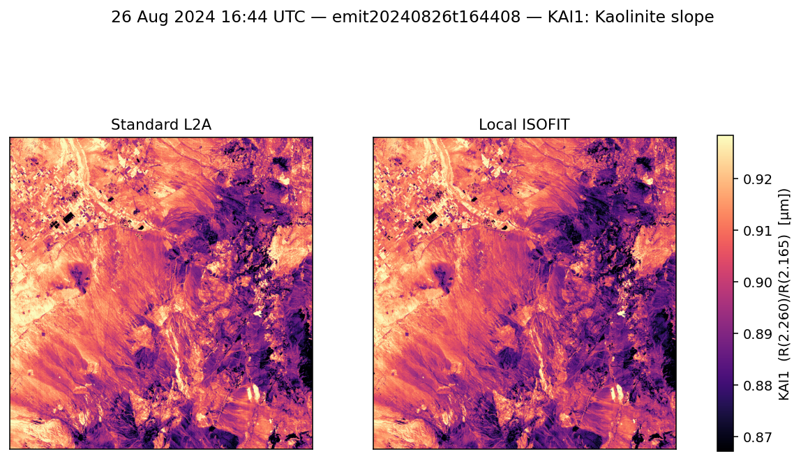
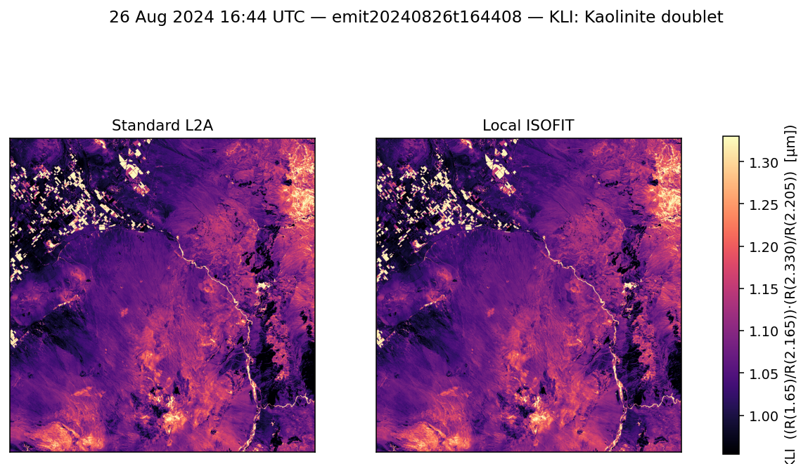
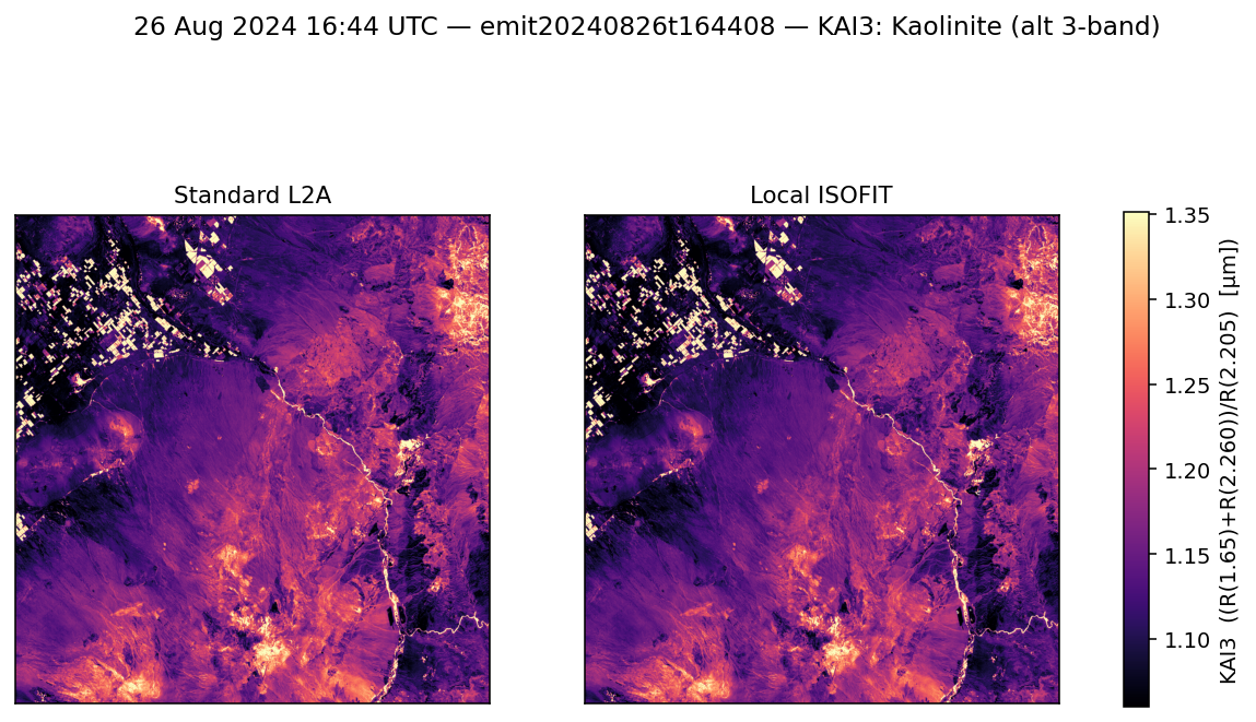
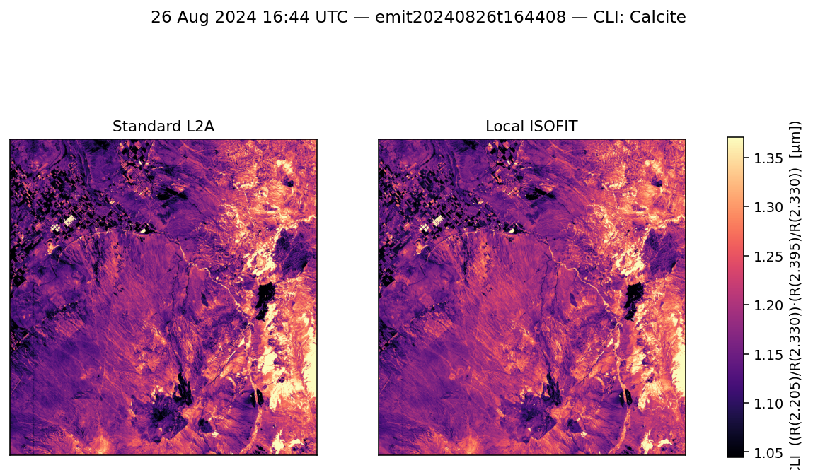
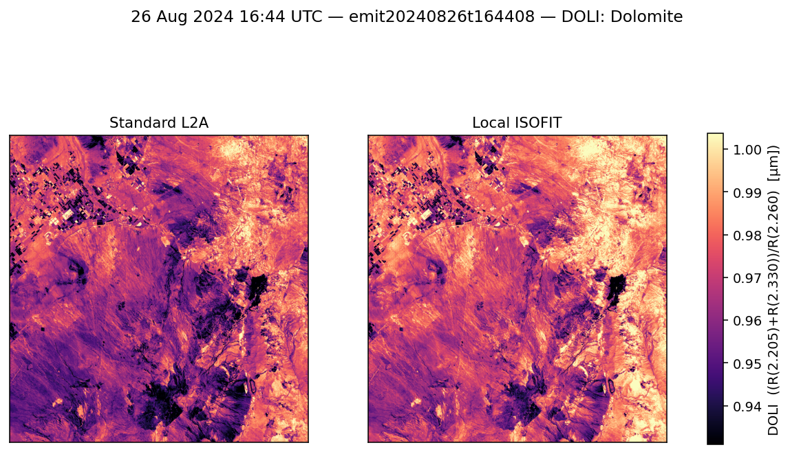
26 Aug 2024 16:44 UTC — emit20240826t164408
Click to expand spectra, PCA grid, eigenvalues, and mineral indices
Mineral spectral indices for 26 Aug 2024 16:44 UTC — emit20240826t164408 (15 maps)
FEAI — Ferric iron alteration
FEI_simple — Ferrous iron
CLAY_TM — Generic clay (TM5/TM7 analog)
CLAI — Argillic alteration (alunite/kaolinite)
ALI — Alunite (Ninomiya)
KAI1 — Kaolinite slope
KLI — Kaolinite doublet
KAI3 — Kaolinite (alt 3-band)
OHI — OH-bearing minerals
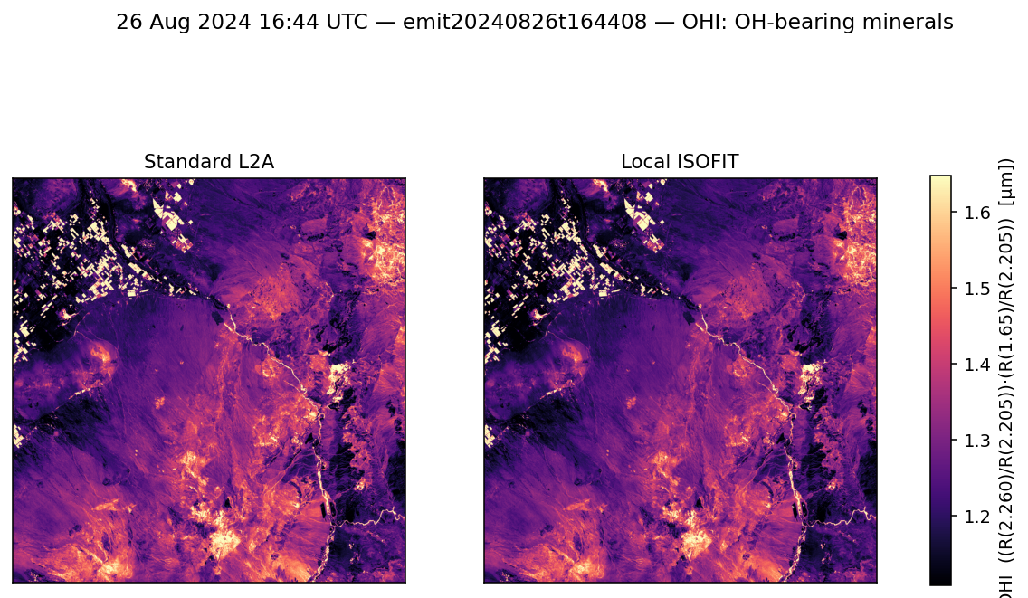
OHI3 — OH near 2.17 µm
CLI — Calcite
DOLI — Dolomite
MGAI — Mg-OH/chlorite/epidote
MONI — Montmorillonite
PRAI — Propylitic alteration
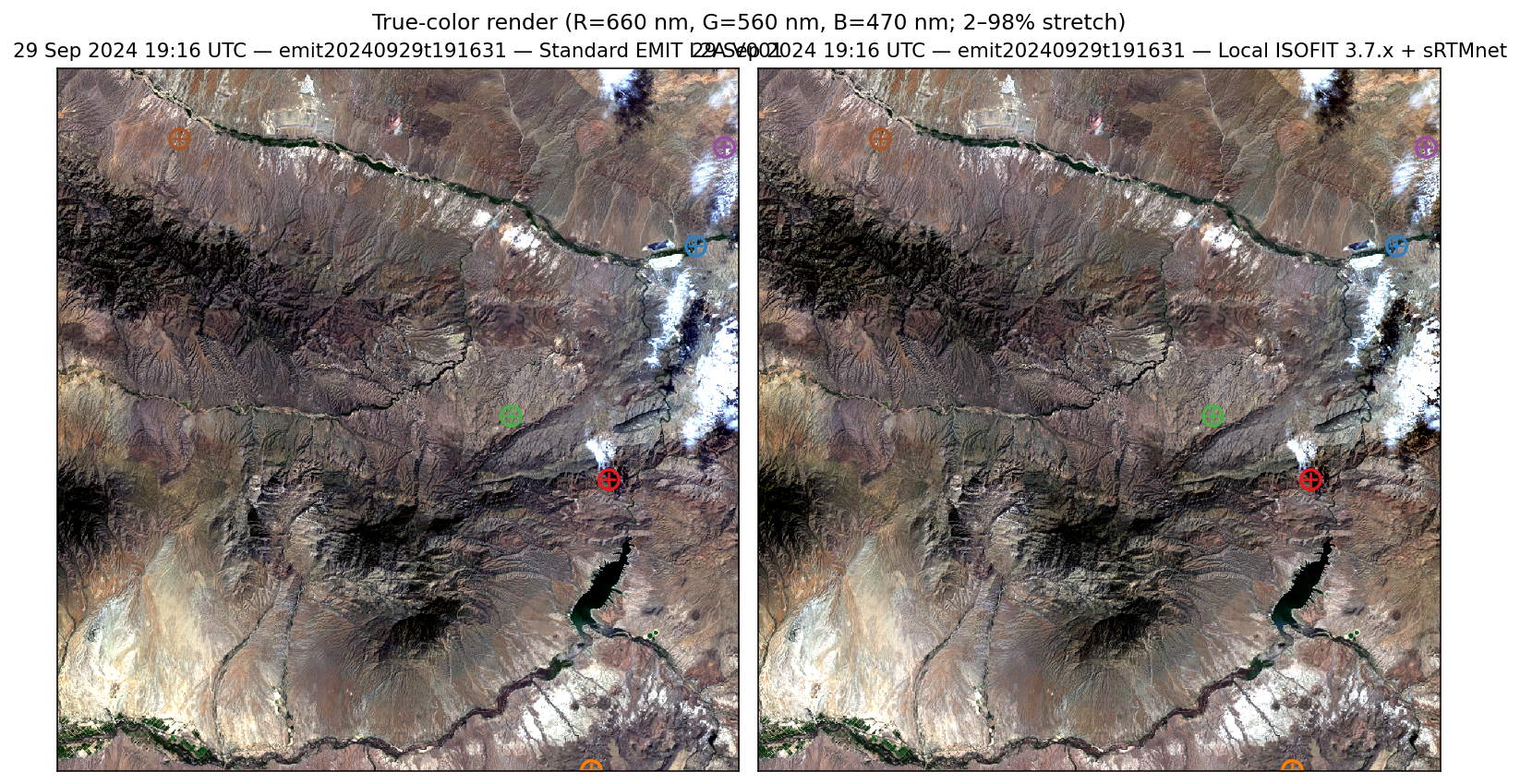
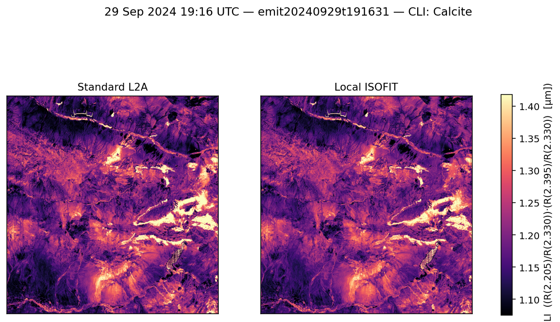
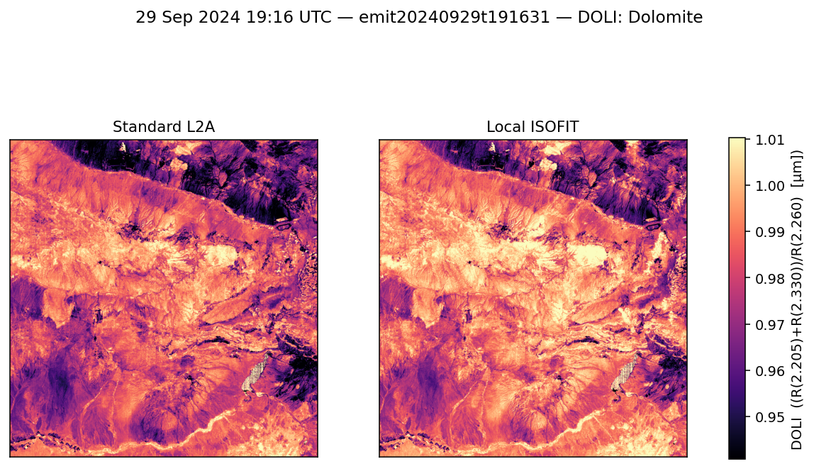
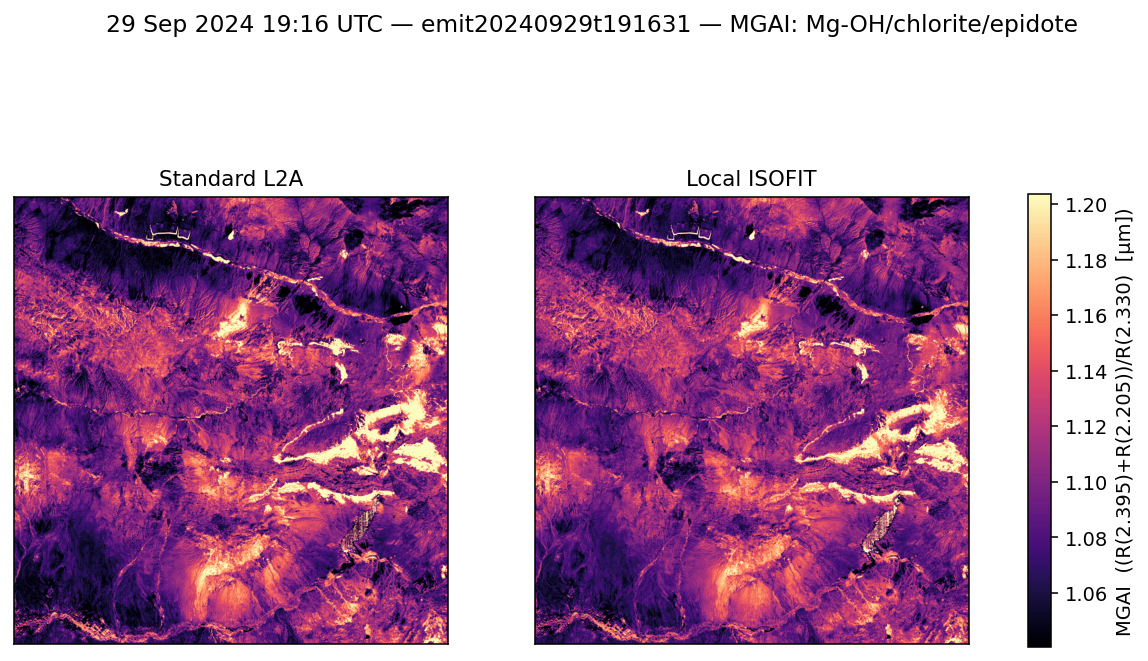
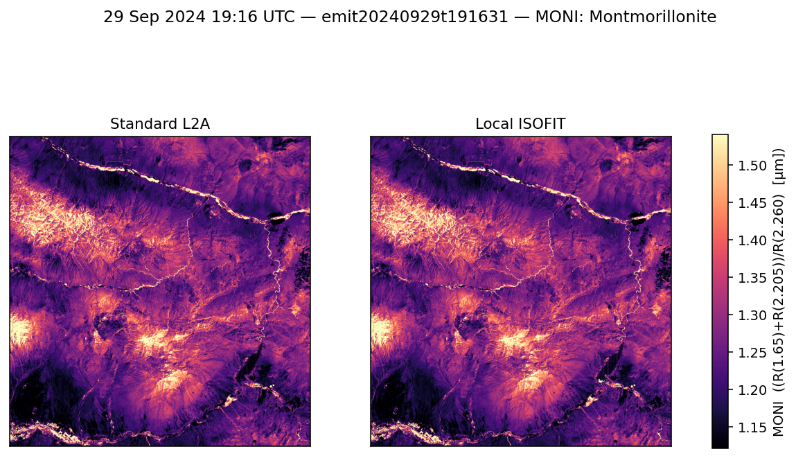
29 Sep 2024 19:16 UTC — emit20240929t191631
Click to expand spectra, PCA grid, eigenvalues, and mineral indices

Mineral spectral indices for 29 Sep 2024 19:16 UTC — emit20240929t191631 (15 maps)
FEAI — Ferric iron alteration
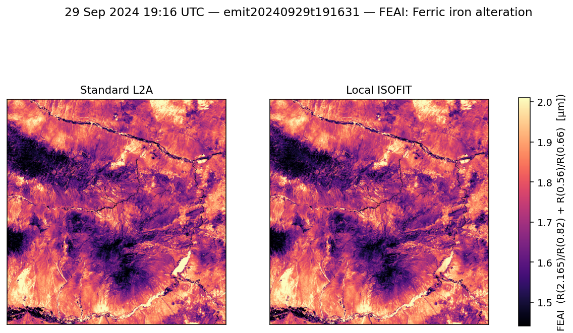
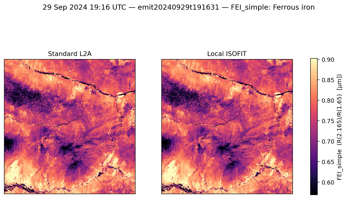
FEI_simple — Ferrous iron
CLAY_TM — Generic clay (TM5/TM7 analog)
CLAI — Argillic alteration (alunite/kaolinite)
ALI — Alunite (Ninomiya)
KAI1 — Kaolinite slope
KLI — Kaolinite doublet
KAI3 — Kaolinite (alt 3-band)
OHI — OH-bearing minerals
OHI3 — OH near 2.17 µm
CLI — Calcite
DOLI — Dolomite
MGAI — Mg-OH/chlorite/epidote
MONI — Montmorillonite
PRAI — Propylitic alteration
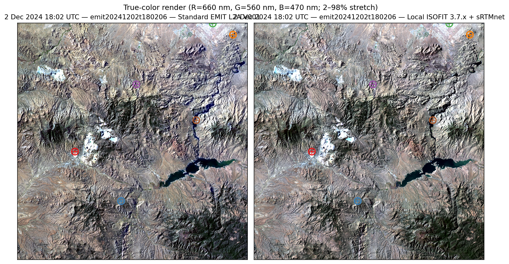
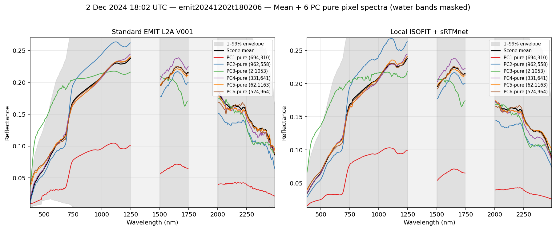
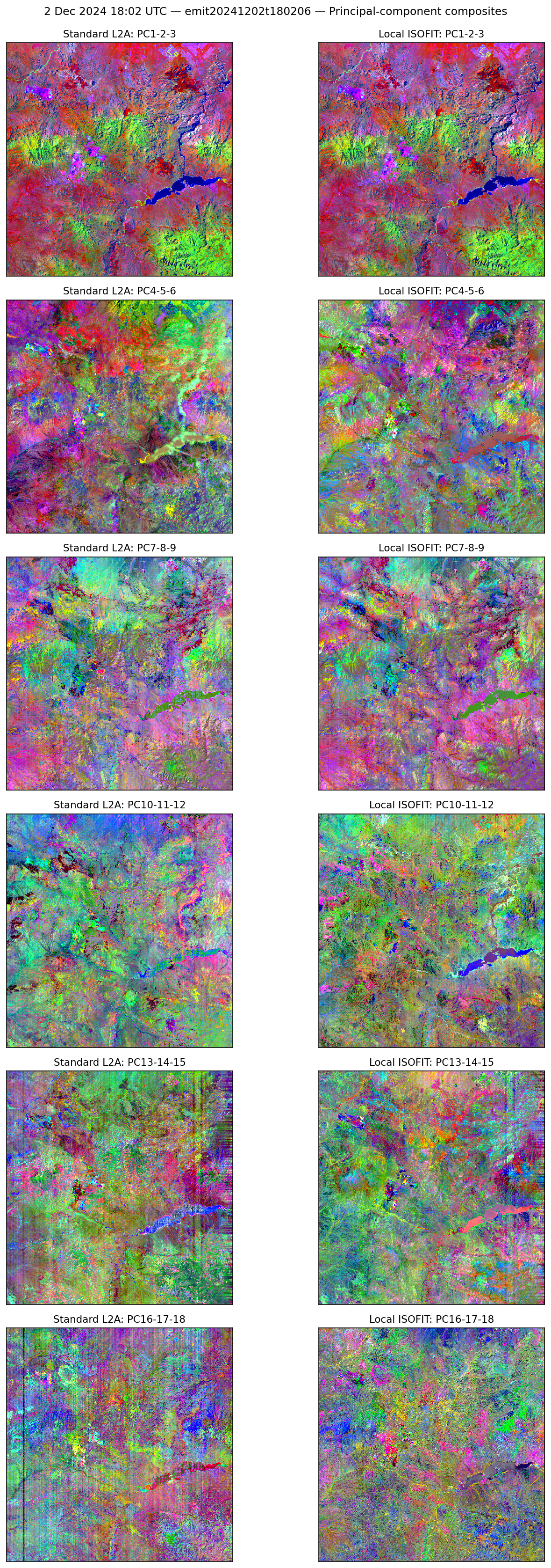
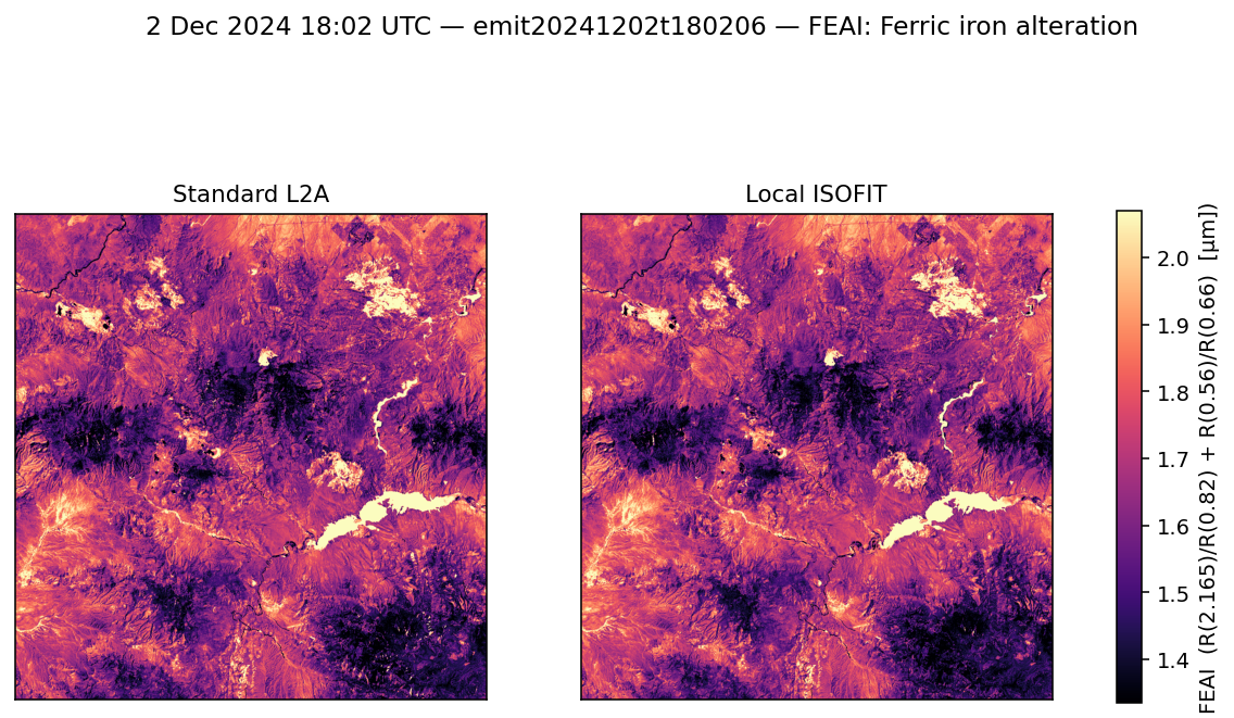
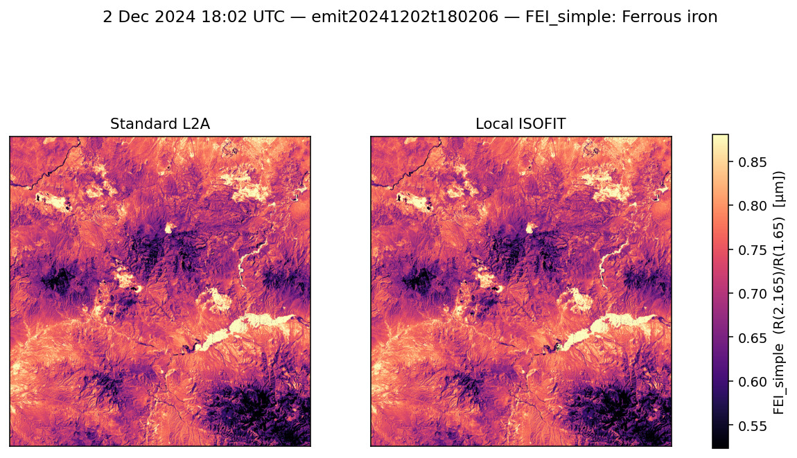
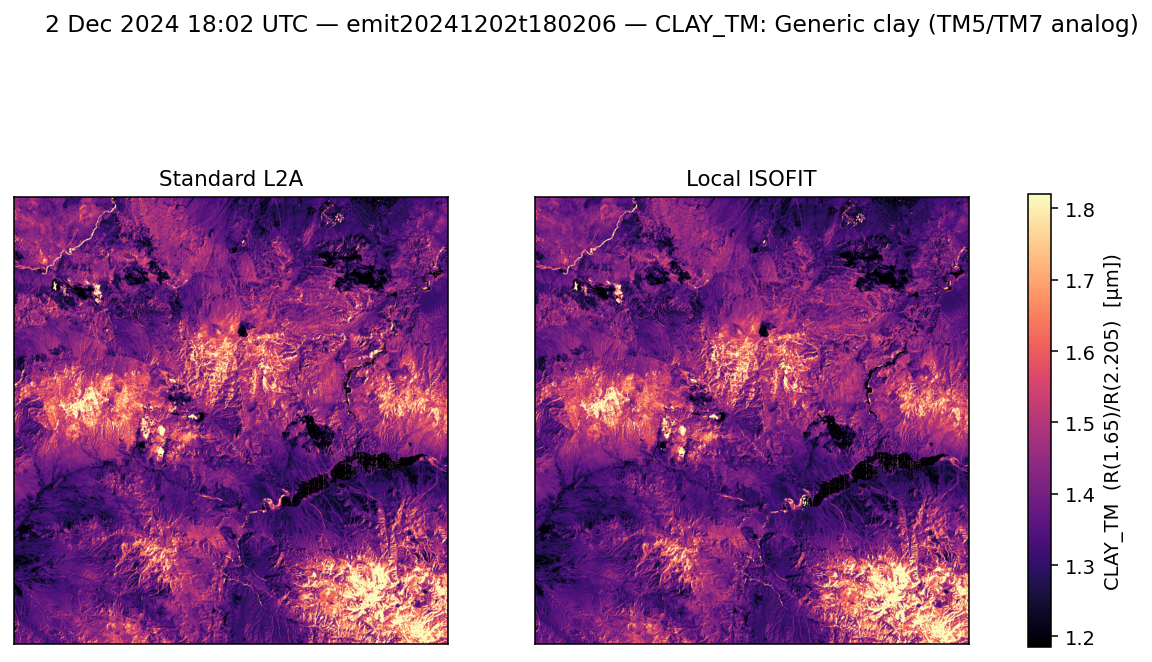
2 Dec 2024 18:02 UTC — emit20241202t180206
Click to expand spectra, PCA grid, eigenvalues, and mineral indices
Mineral spectral indices for 2 Dec 2024 18:02 UTC — emit20241202t180206 (15 maps)
FEAI — Ferric iron alteration
FEI_simple — Ferrous iron
CLAY_TM — Generic clay (TM5/TM7 analog)
CLAI — Argillic alteration (alunite/kaolinite)
ALI — Alunite (Ninomiya)
KAI1 — Kaolinite slope
KLI — Kaolinite doublet
KAI3 — Kaolinite (alt 3-band)
OHI — OH-bearing minerals
OHI3 — OH near 2.17 µm
CLI — Calcite
DOLI — Dolomite
MGAI — Mg-OH/chlorite/epidote
MONI — Montmorillonite
PRAI — Propylitic alteration
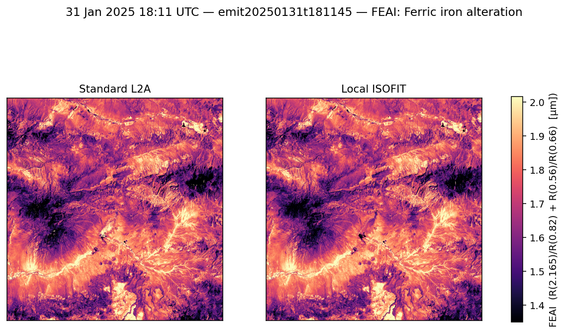
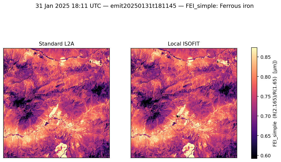
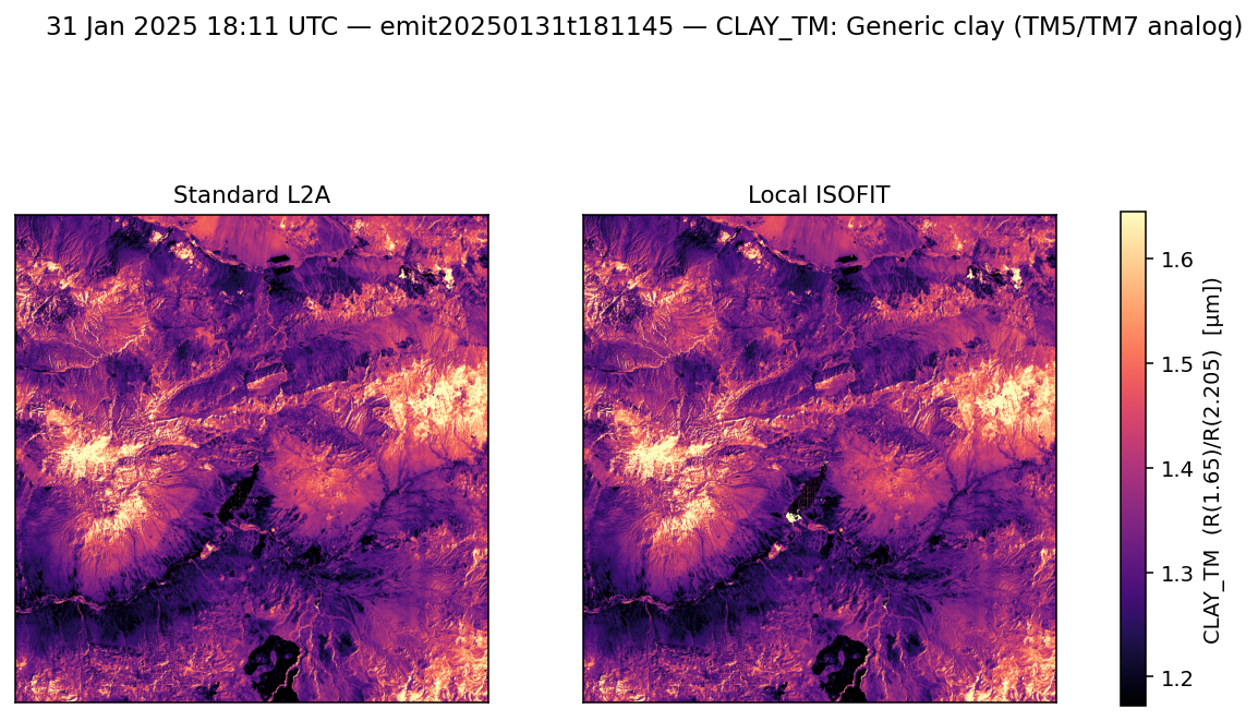
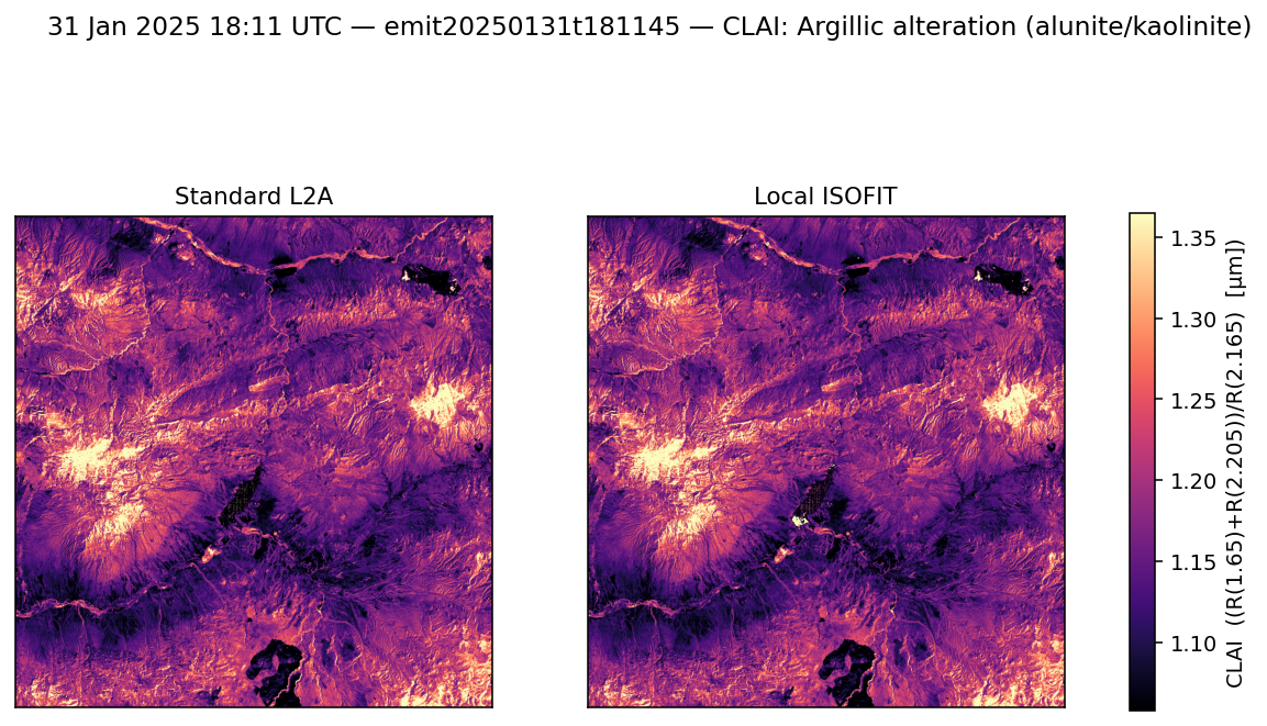
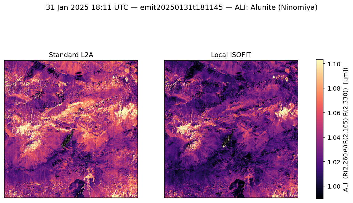
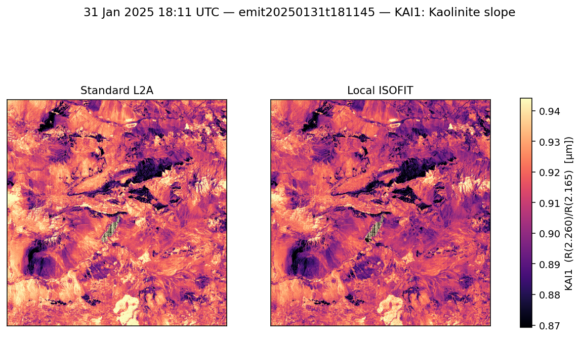
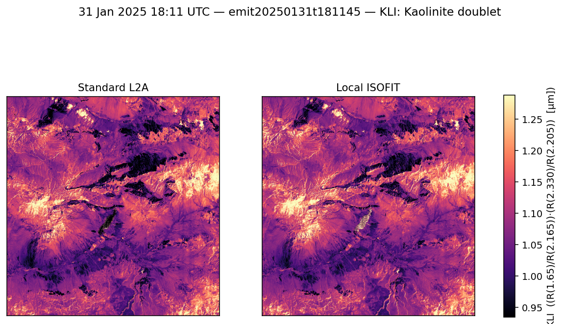
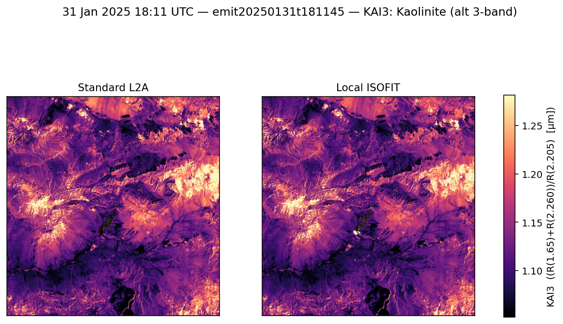
31 Jan 2025 18:11 UTC — emit20250131t181145
Click to expand spectra, PCA grid, eigenvalues, and mineral indices
Mineral spectral indices for 31 Jan 2025 18:11 UTC — emit20250131t181145 (15 maps)
FEAI — Ferric iron alteration
FEI_simple — Ferrous iron
CLAY_TM — Generic clay (TM5/TM7 analog)
CLAI — Argillic alteration (alunite/kaolinite)
ALI — Alunite (Ninomiya)
KAI1 — Kaolinite slope
KLI — Kaolinite doublet
KAI3 — Kaolinite (alt 3-band)
OHI — OH-bearing minerals
OHI3 — OH near 2.17 µm
CLI — Calcite
DOLI — Dolomite
MGAI — Mg-OH/chlorite/epidote
MONI — Montmorillonite
PRAI — Propylitic alteration
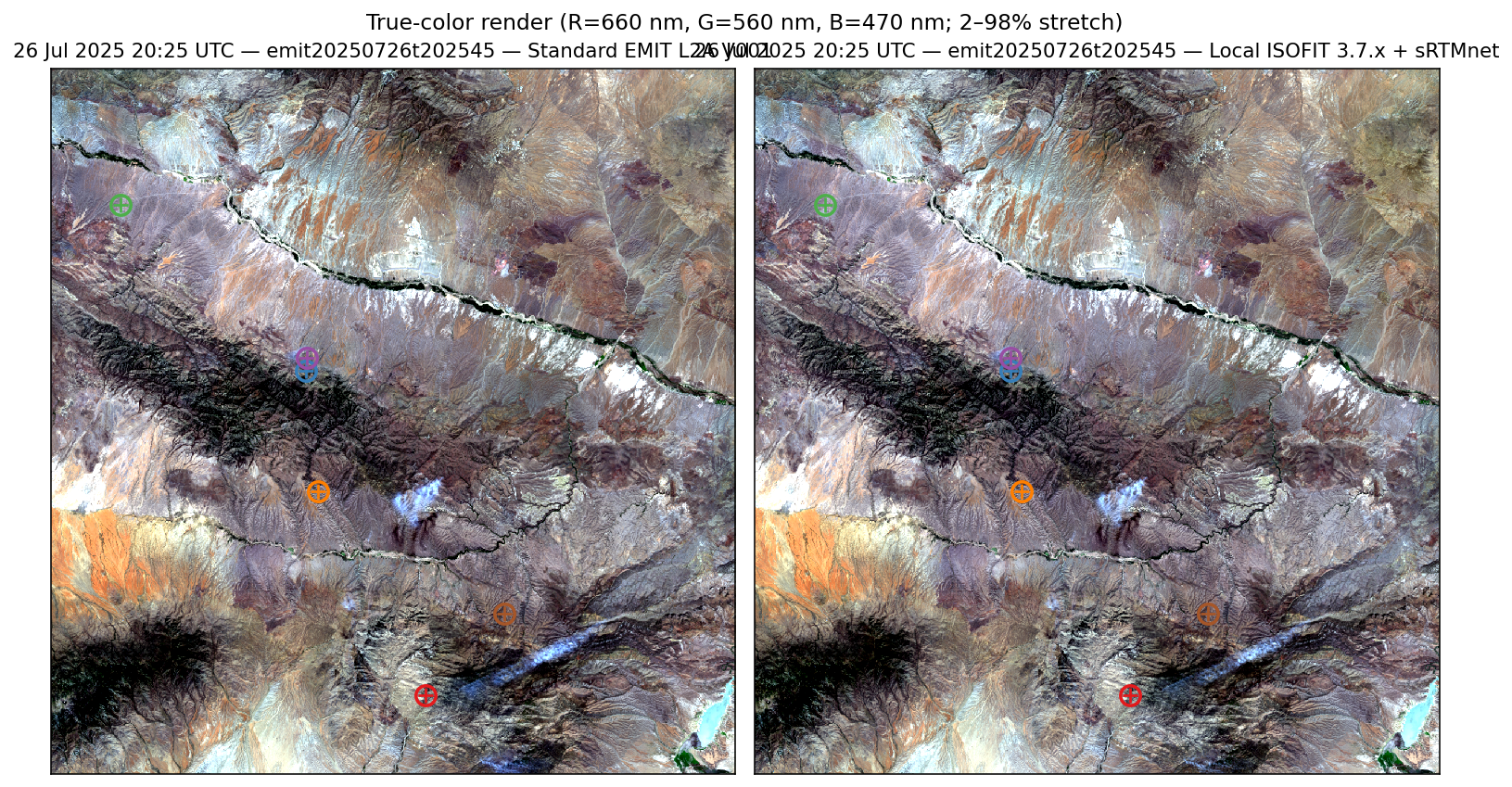
26 Jul 2025 20:25 UTC — emit20250726t202545
Click to expand spectra, PCA grid, eigenvalues, and mineral indices

Mineral spectral indices for 26 Jul 2025 20:25 UTC — emit20250726t202545 (15 maps)
FEAI — Ferric iron alteration
FEI_simple — Ferrous iron
CLAY_TM — Generic clay (TM5/TM7 analog)
CLAI — Argillic alteration (alunite/kaolinite)
ALI — Alunite (Ninomiya)
KAI1 — Kaolinite slope
KLI — Kaolinite doublet
KAI3 — Kaolinite (alt 3-band)
OHI — OH-bearing minerals
OHI3 — OH near 2.17 µm
CLI — Calcite
DOLI — Dolomite
MGAI — Mg-OH/chlorite/epidote
MONI — Montmorillonite
PRAI — Propylitic alteration
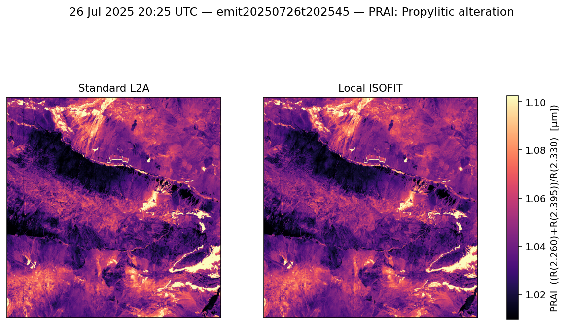
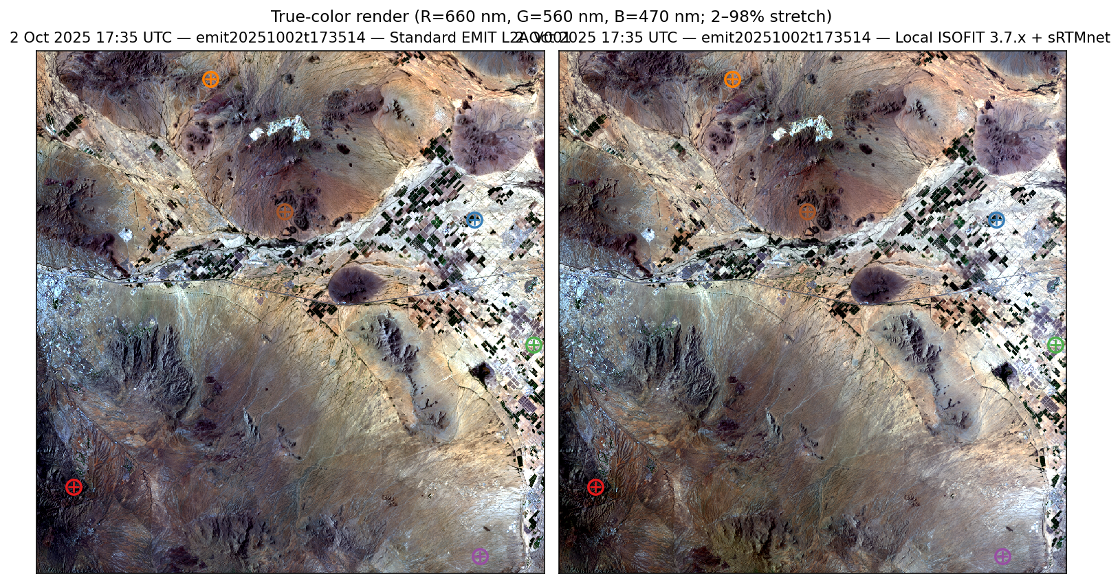
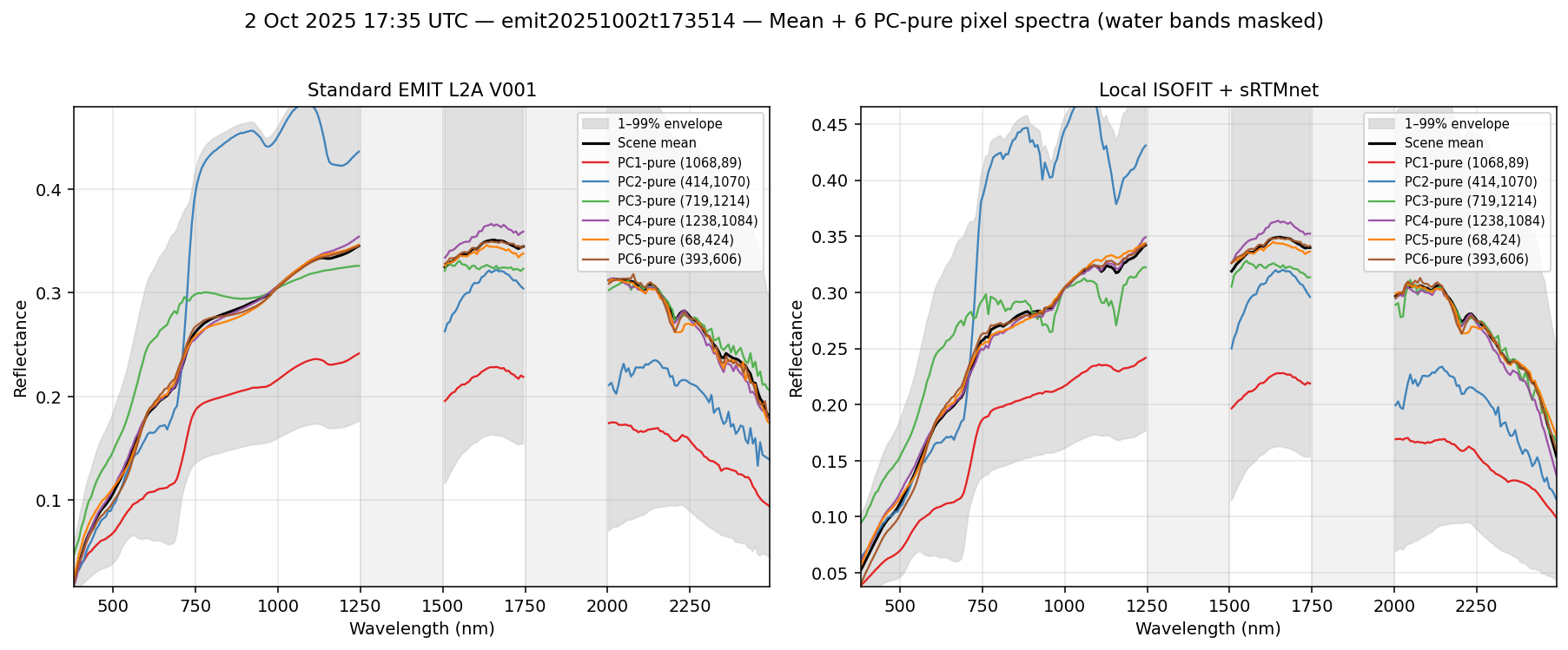
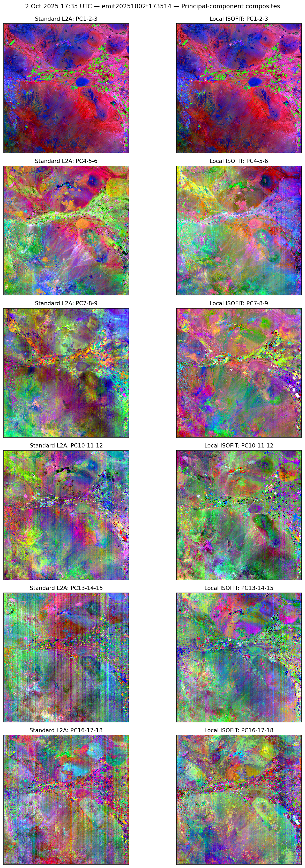
2 Oct 2025 17:35 UTC — emit20251002t173514
Click to expand spectra, PCA grid, eigenvalues, and mineral indices
Mineral spectral indices for 2 Oct 2025 17:35 UTC — emit20251002t173514 (15 maps)
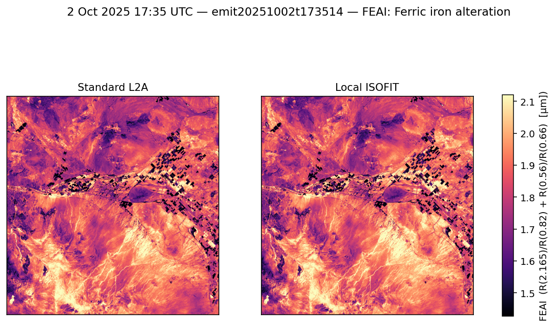
FEAI — Ferric iron alteration
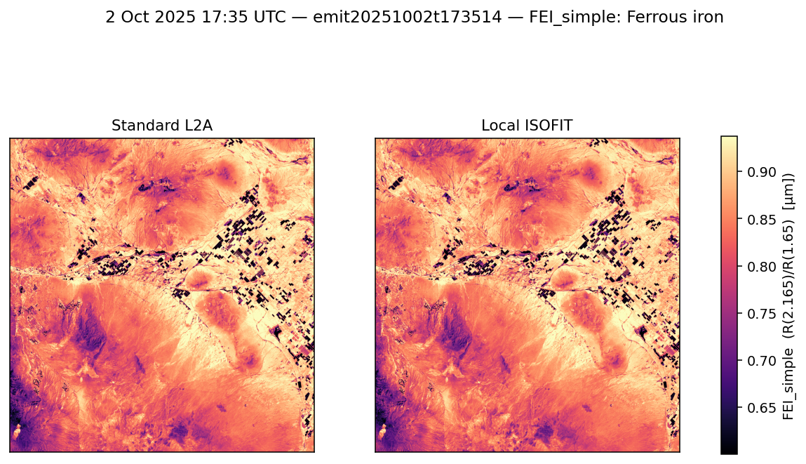
FEI_simple — Ferrous iron
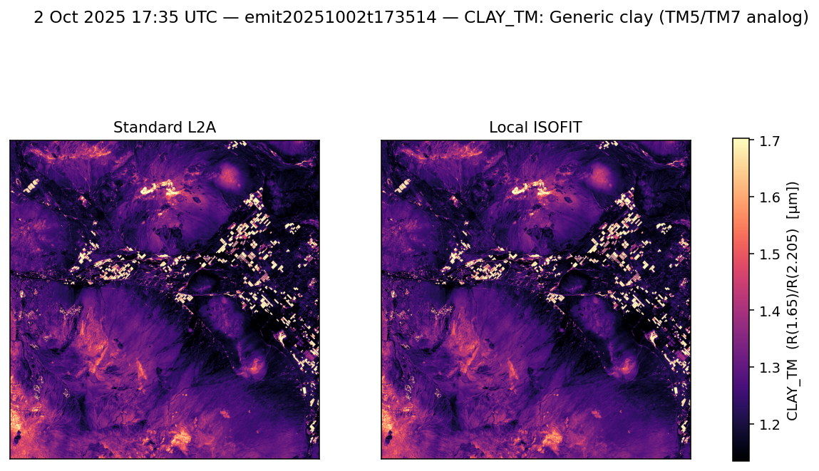
CLAY_TM — Generic clay (TM5/TM7 analog)
CLAI — Argillic alteration (alunite/kaolinite)
ALI — Alunite (Ninomiya)
KAI1 — Kaolinite slope
KLI — Kaolinite doublet
KAI3 — Kaolinite (alt 3-band)
OHI — OH-bearing minerals
OHI3 — OH near 2.17 µm
CLI — Calcite
DOLI — Dolomite
MGAI — Mg-OH/chlorite/epidote
MONI — Montmorillonite
PRAI — Propylitic alteration
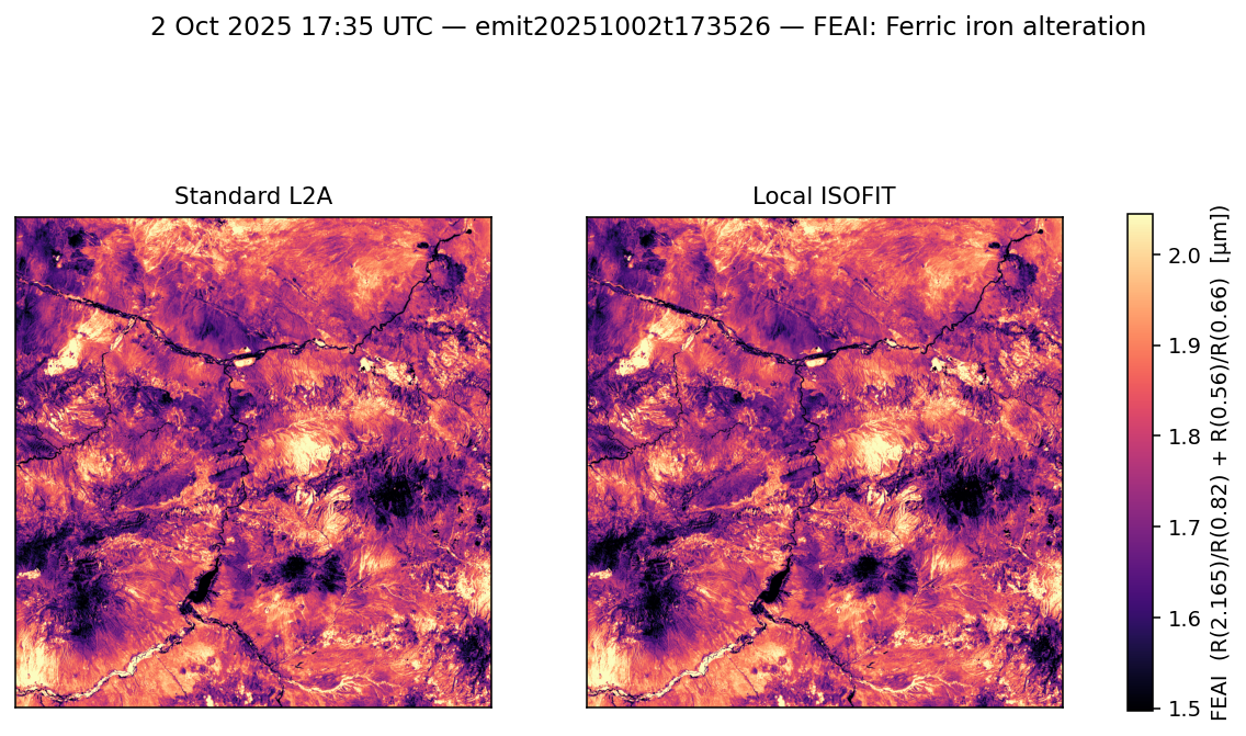
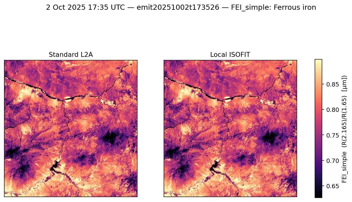
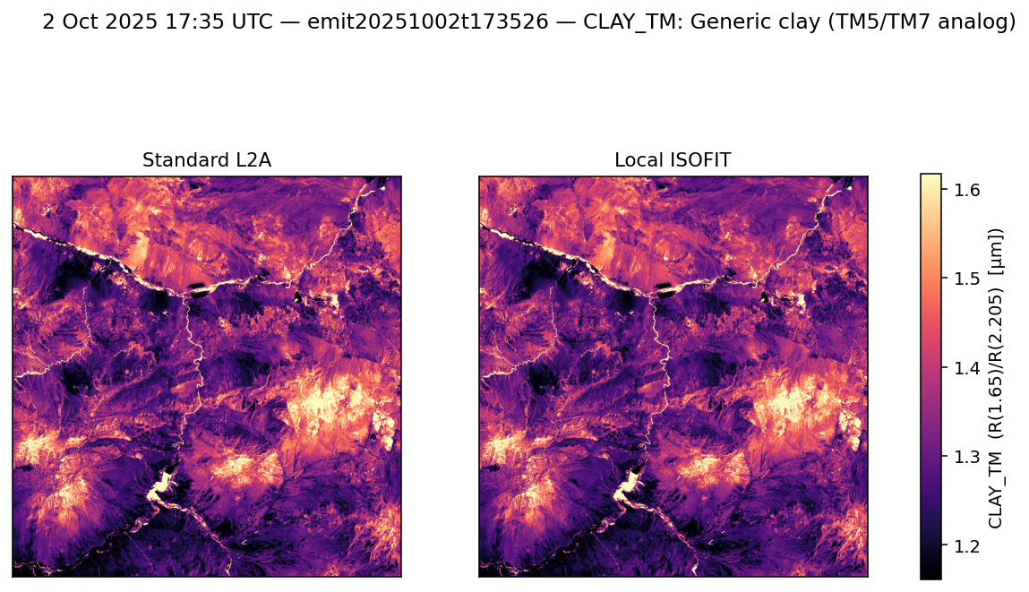
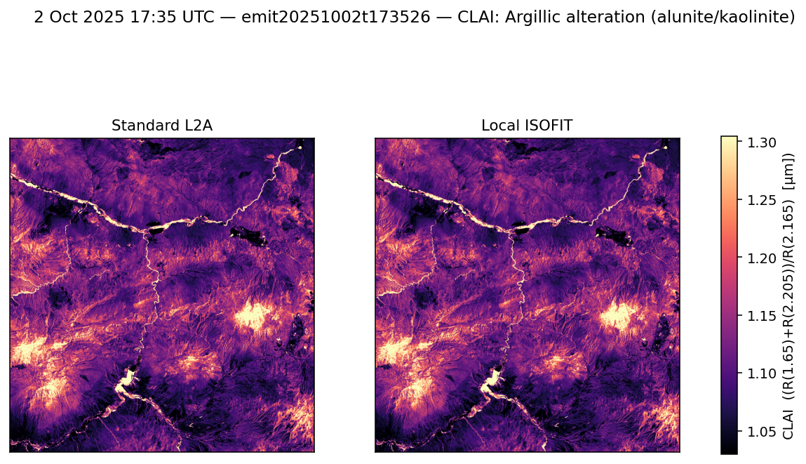
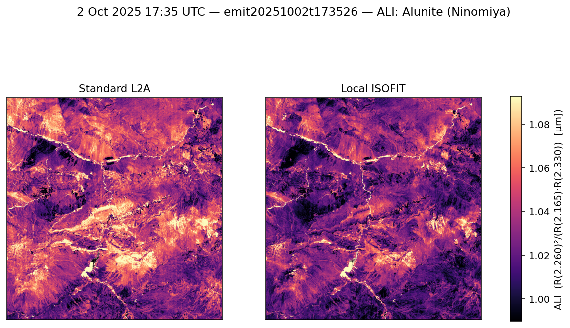
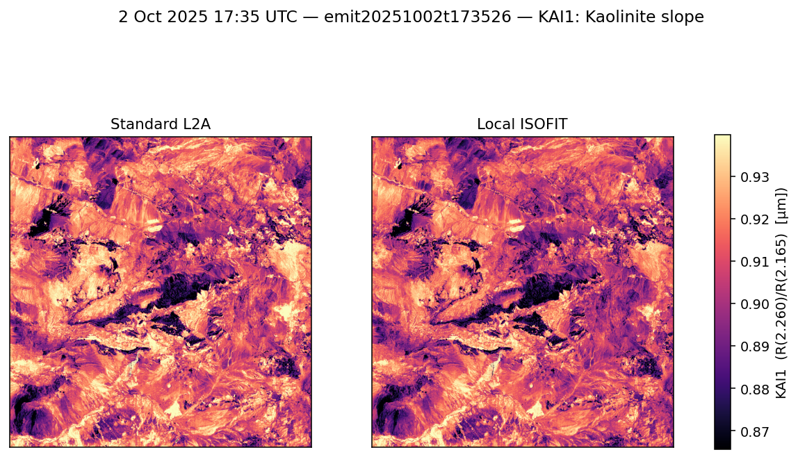
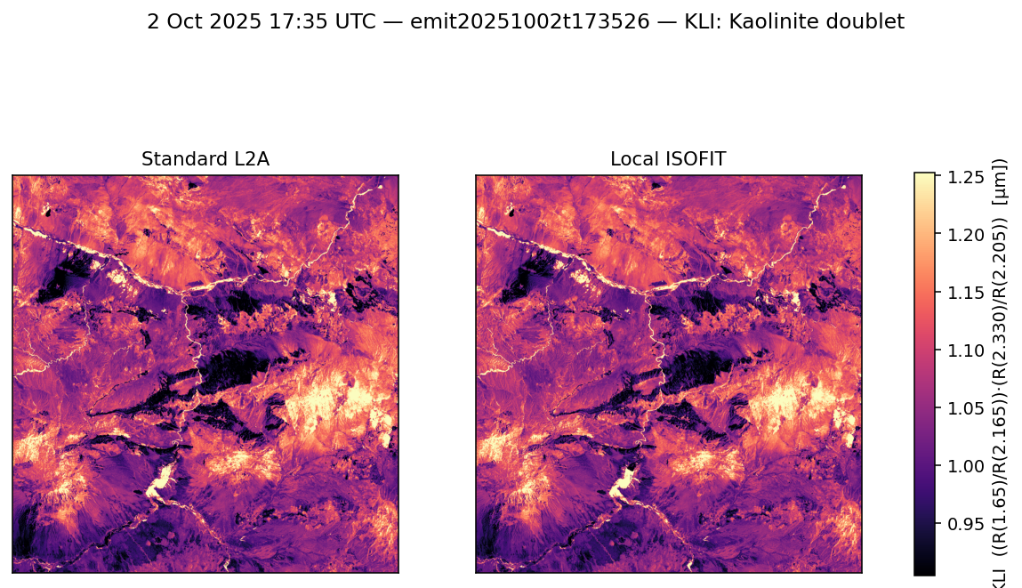
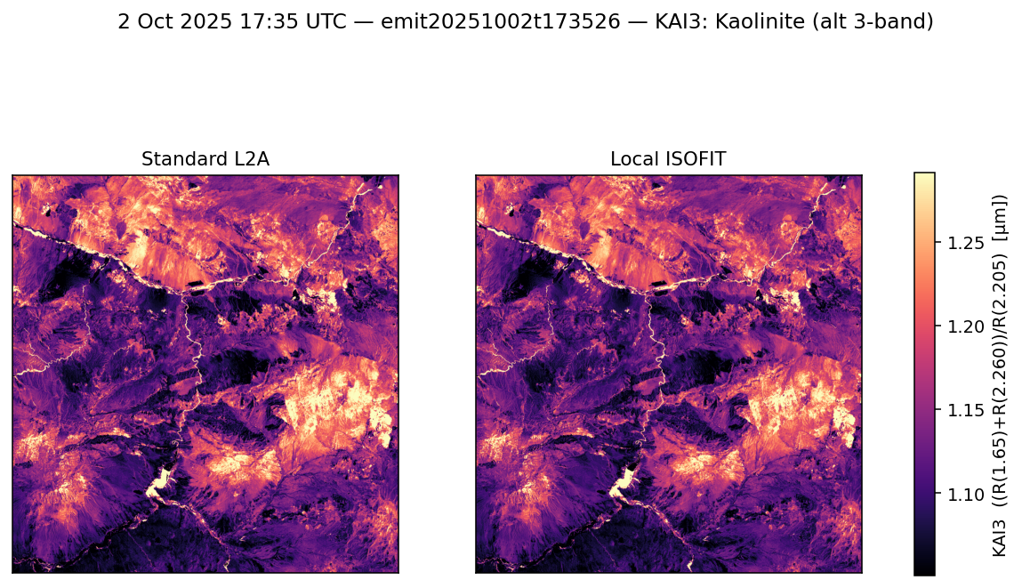
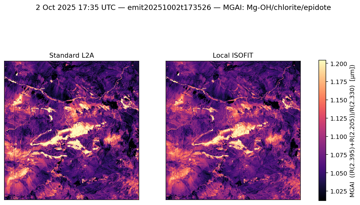
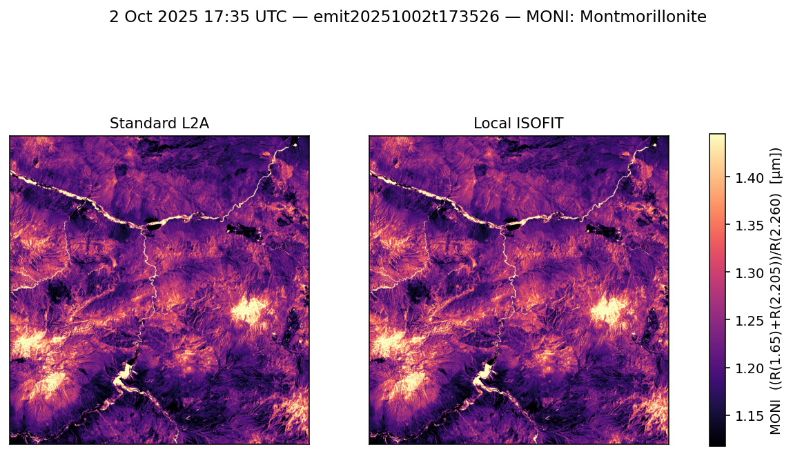
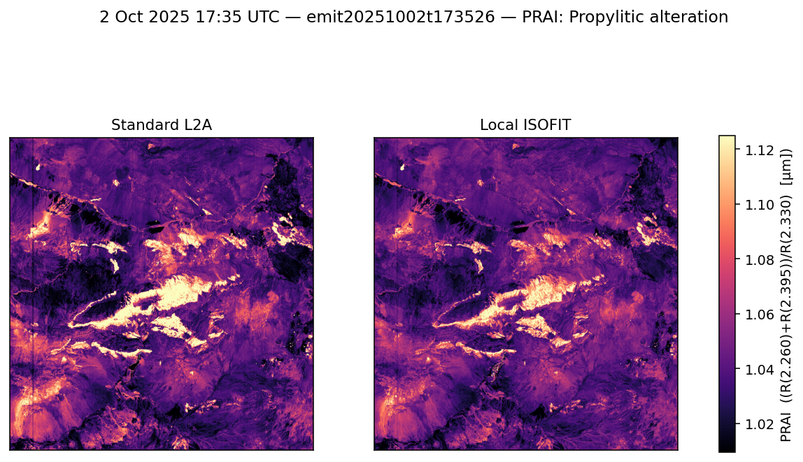
2 Oct 2025 17:35 UTC — emit20251002t173526
Click to expand spectra, PCA grid, eigenvalues, and mineral indices
Mineral spectral indices for 2 Oct 2025 17:35 UTC — emit20251002t173526 (15 maps)
FEAI — Ferric iron alteration
FEI_simple — Ferrous iron
CLAY_TM — Generic clay (TM5/TM7 analog)
CLAI — Argillic alteration (alunite/kaolinite)
ALI — Alunite (Ninomiya)
KAI1 — Kaolinite slope
KLI — Kaolinite doublet
KAI3 — Kaolinite (alt 3-band)
OHI — OH-bearing minerals
OHI3 — OH near 2.17 µm
CLI — Calcite
DOLI — Dolomite
MGAI — Mg-OH/chlorite/epidote
MONI — Montmorillonite
PRAI — Propylitic alteration
Tier 2 — Mild Cloud Fraction Included in Processing 3 scenes
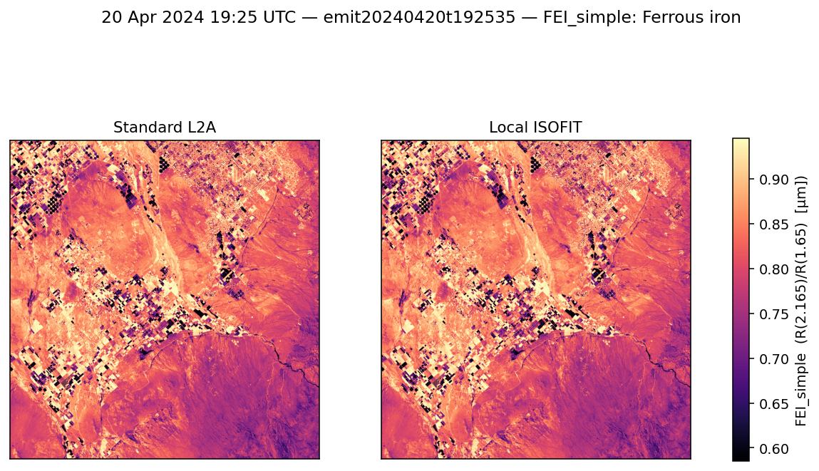
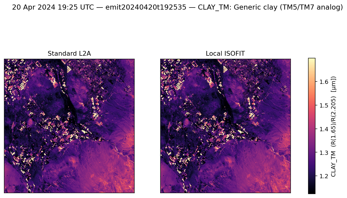
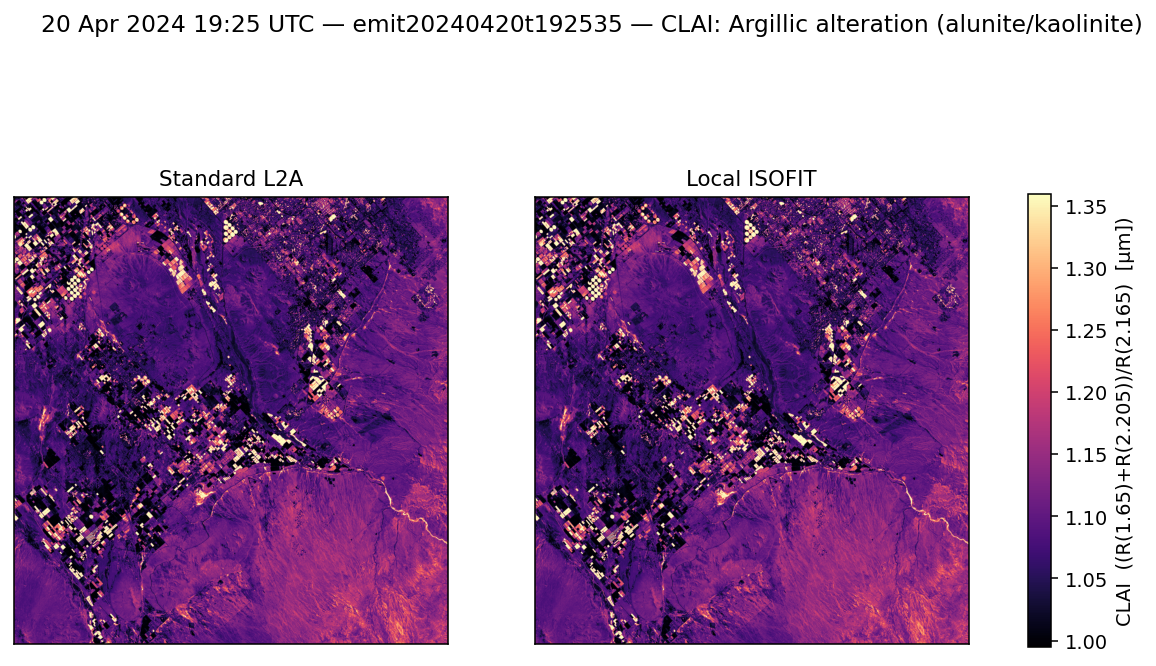
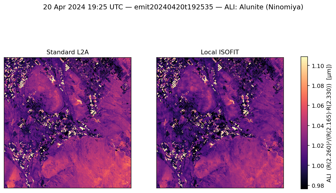
20 Apr 2024 19:25 UTC — emit20240420t192535Tier 2 — flagged: 12.4% cloud
Click to expand spectra, PCA grid, eigenvalues, and mineral indices
Mineral spectral indices for 20 Apr 2024 19:25 UTC — emit20240420t192535 (15 maps)
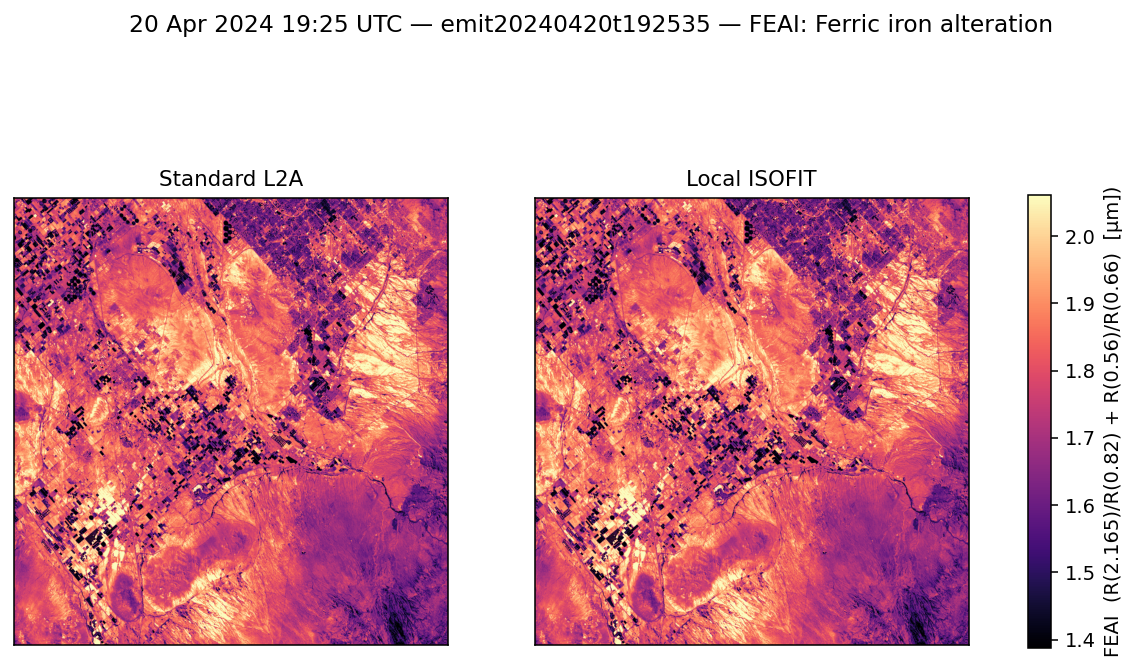
FEAI — Ferric iron alteration
FEI_simple — Ferrous iron
CLAY_TM — Generic clay (TM5/TM7 analog)
CLAI — Argillic alteration (alunite/kaolinite)
ALI — Alunite (Ninomiya)
KAI1 — Kaolinite slope
KLI — Kaolinite doublet
KAI3 — Kaolinite (alt 3-band)
OHI — OH-bearing minerals
OHI3 — OH near 2.17 µm
CLI — Calcite
DOLI — Dolomite
MGAI — Mg-OH/chlorite/epidote
MONI — Montmorillonite
PRAI — Propylitic alteration
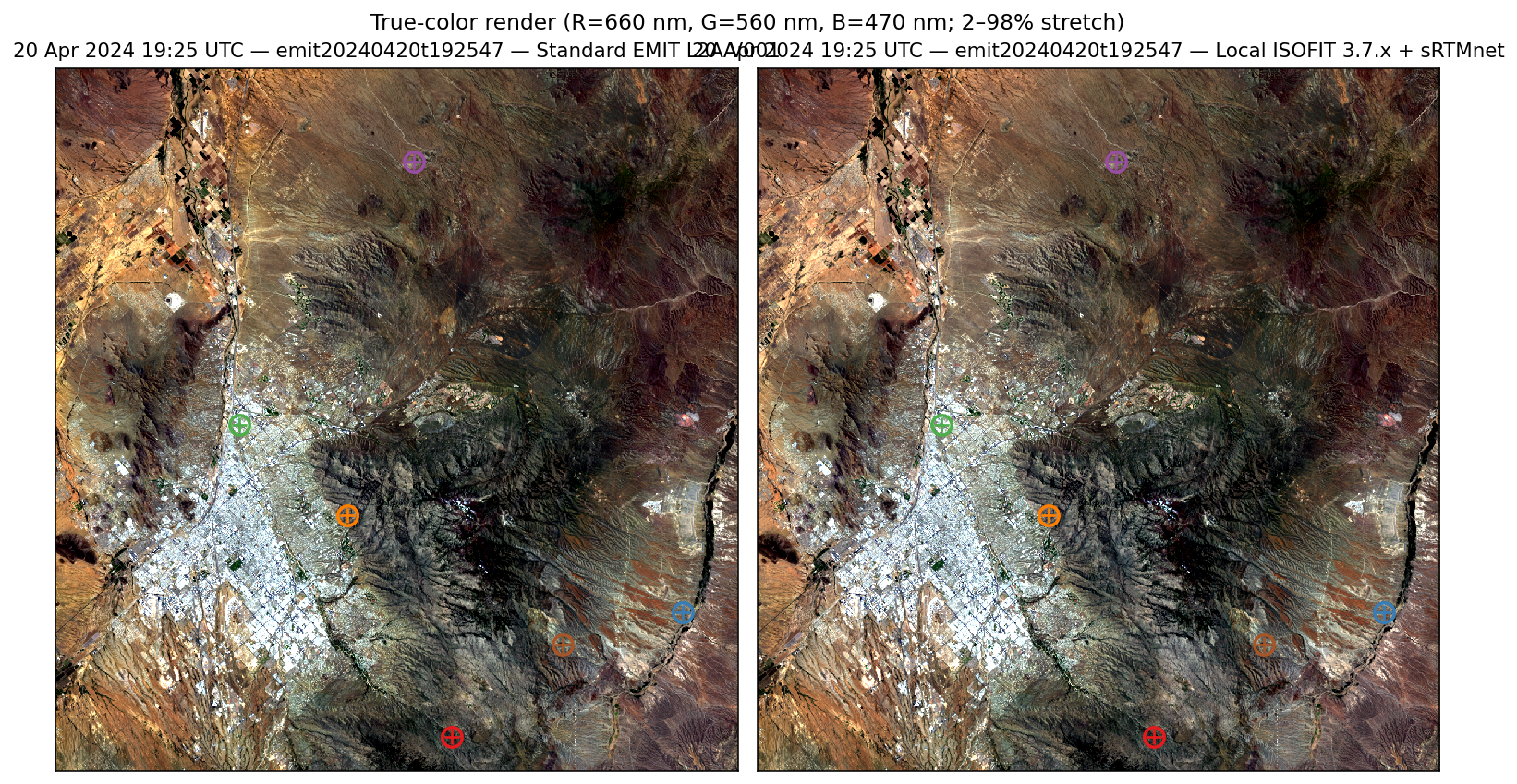
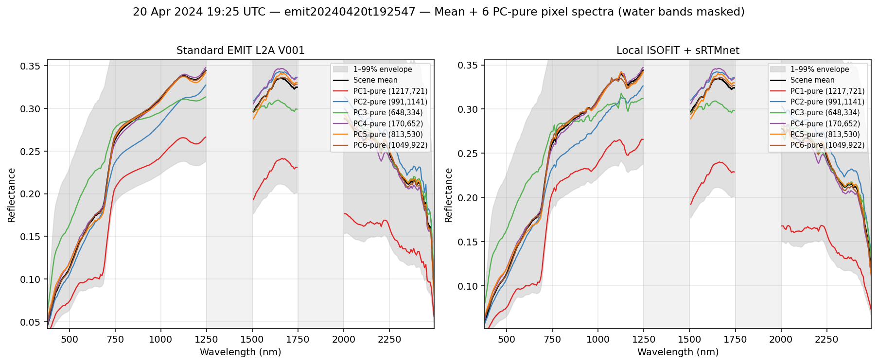
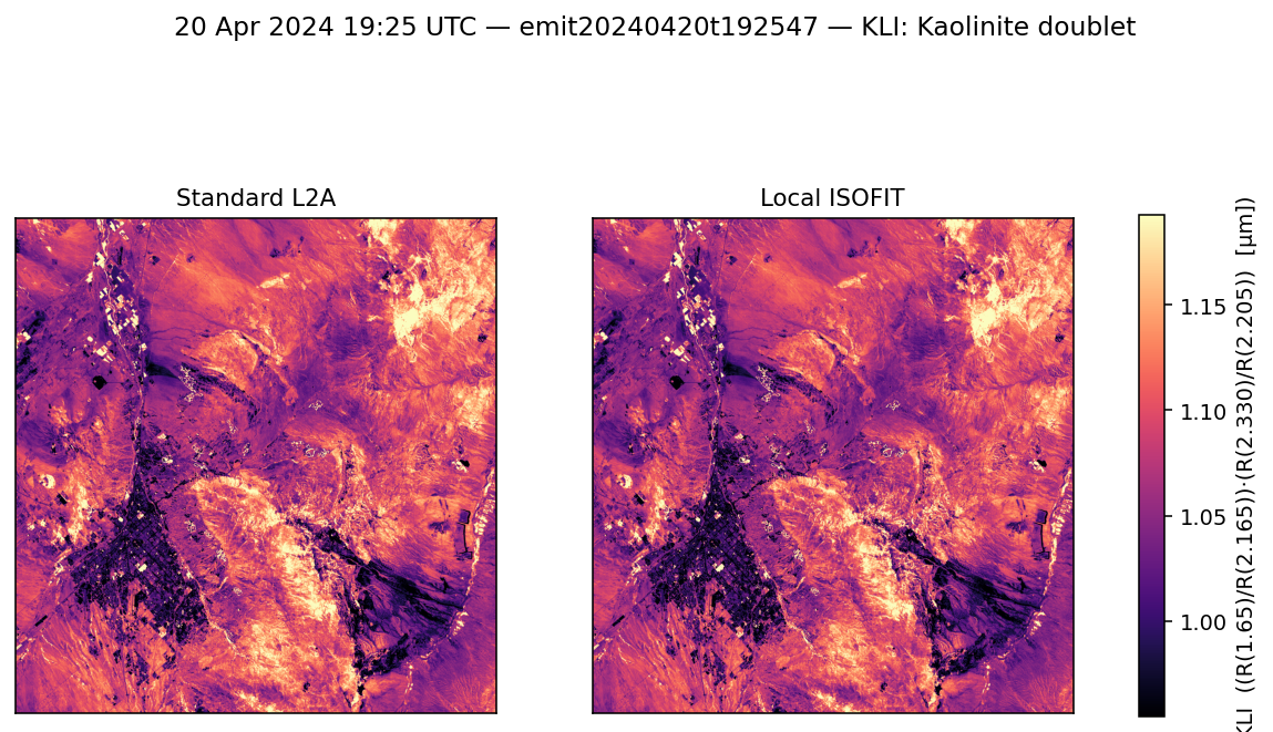
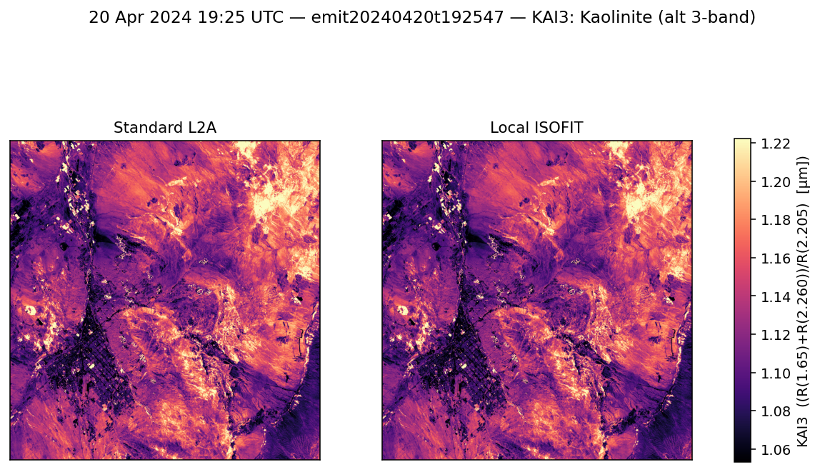
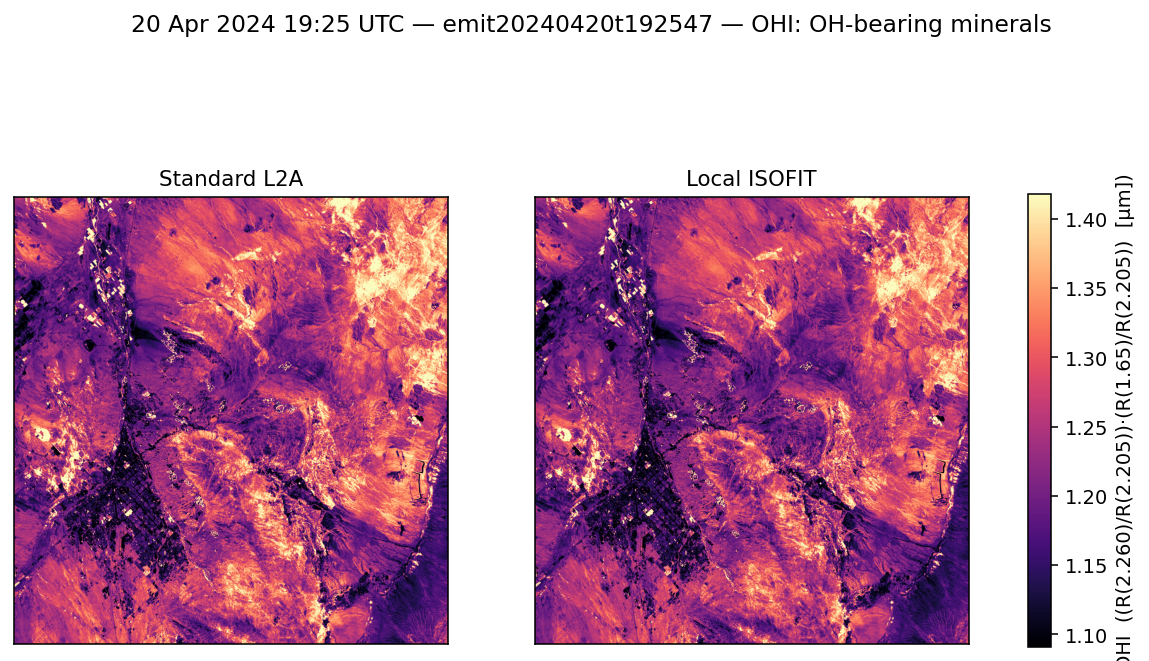
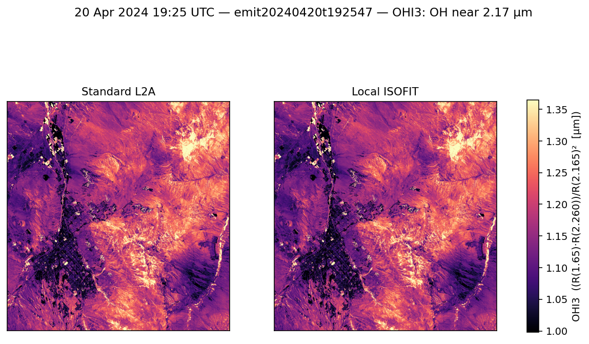
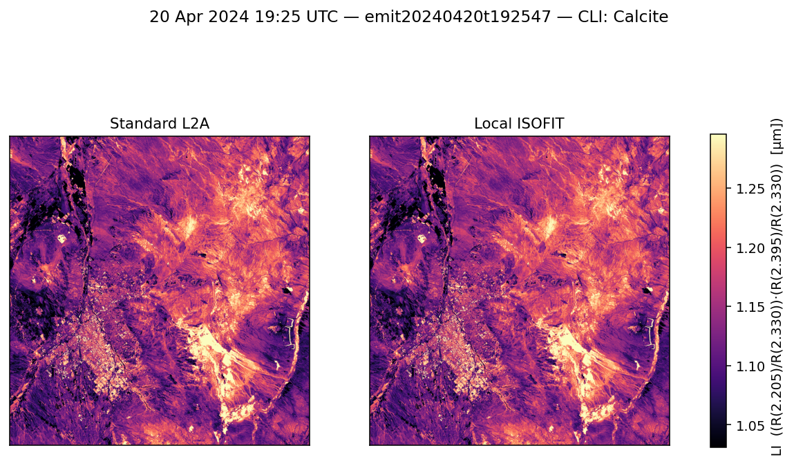
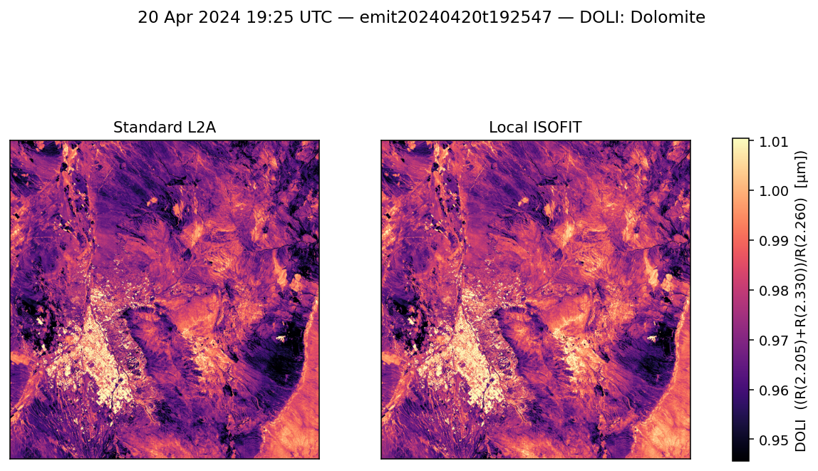
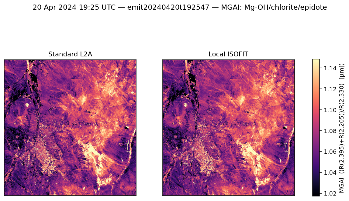
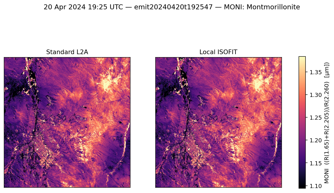
20 Apr 2024 19:25 UTC — emit20240420t192547Tier 2 — flagged: 11.8% cloud
Click to expand spectra, PCA grid, eigenvalues, and mineral indices
Mineral spectral indices for 20 Apr 2024 19:25 UTC — emit20240420t192547 (15 maps)
FEAI — Ferric iron alteration
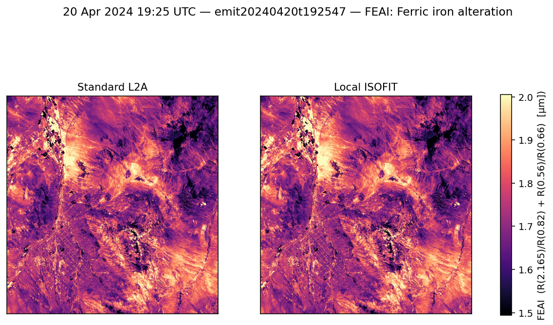
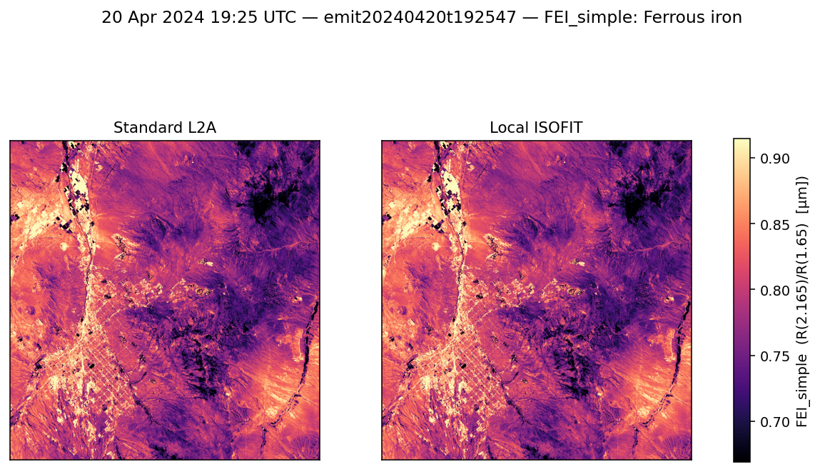
FEI_simple — Ferrous iron
CLAY_TM — Generic clay (TM5/TM7 analog)
CLAI — Argillic alteration (alunite/kaolinite)
ALI — Alunite (Ninomiya)
KAI1 — Kaolinite slope
KLI — Kaolinite doublet
KAI3 — Kaolinite (alt 3-band)
OHI — OH-bearing minerals
OHI3 — OH near 2.17 µm
CLI — Calcite
DOLI — Dolomite
MGAI — Mg-OH/chlorite/epidote
MONI — Montmorillonite
PRAI — Propylitic alteration
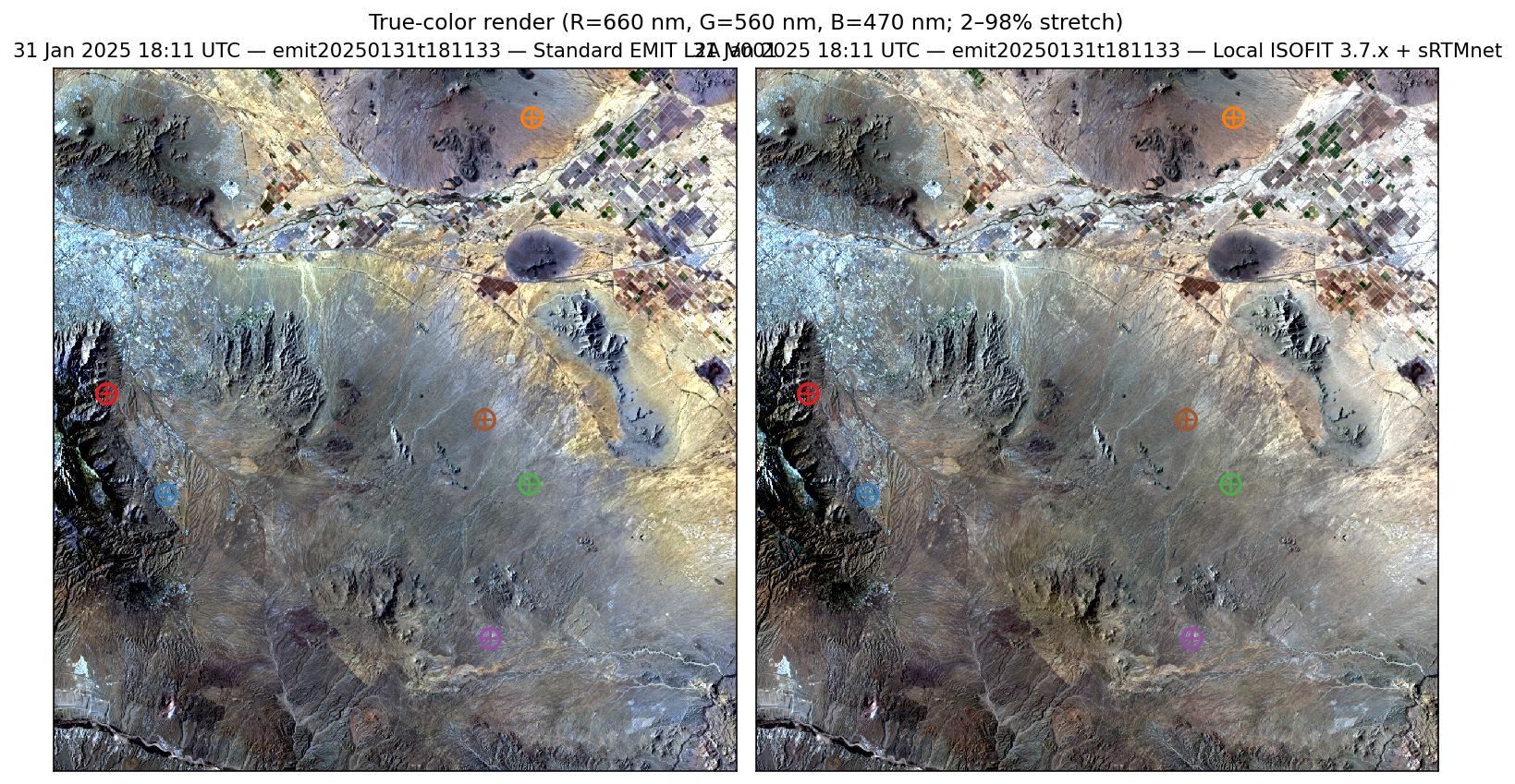
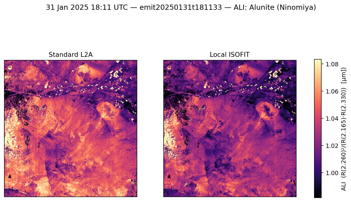
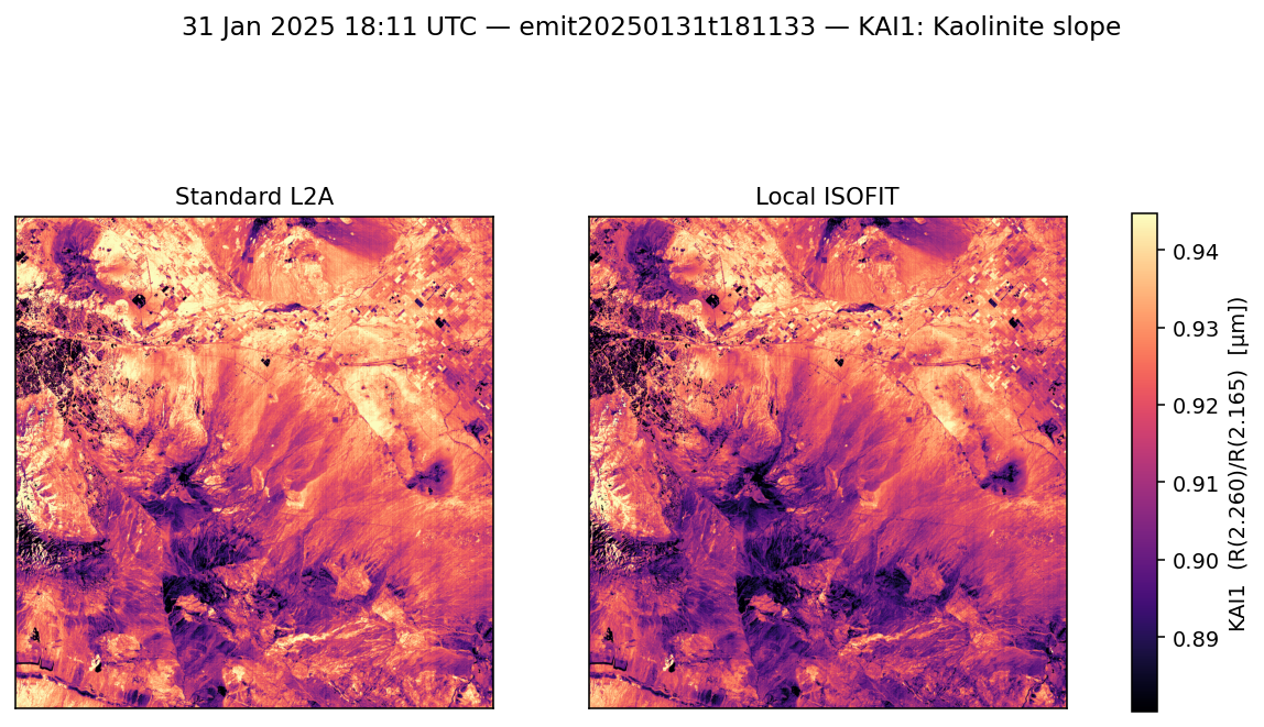
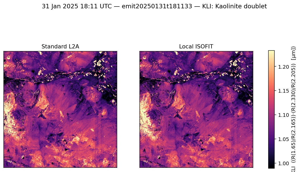
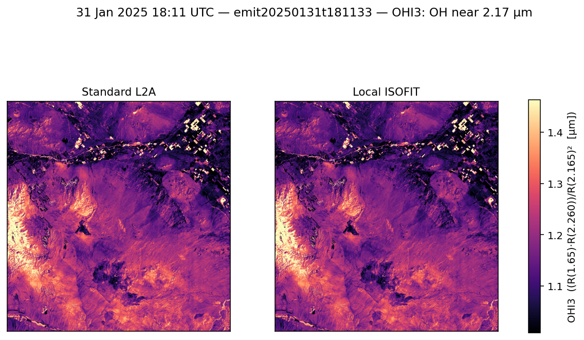
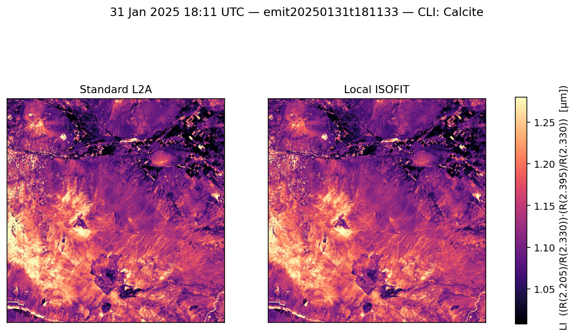
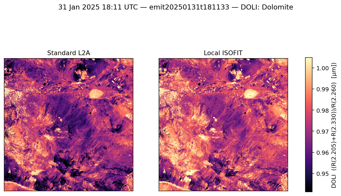
31 Jan 2025 18:11 UTC — emit20250131t181133Tier 2 — flagged: 14.1% cloud
Click to expand spectra, PCA grid, eigenvalues, and mineral indices
Mineral spectral indices for 31 Jan 2025 18:11 UTC — emit20250131t181133 (15 maps)
FEAI — Ferric iron alteration
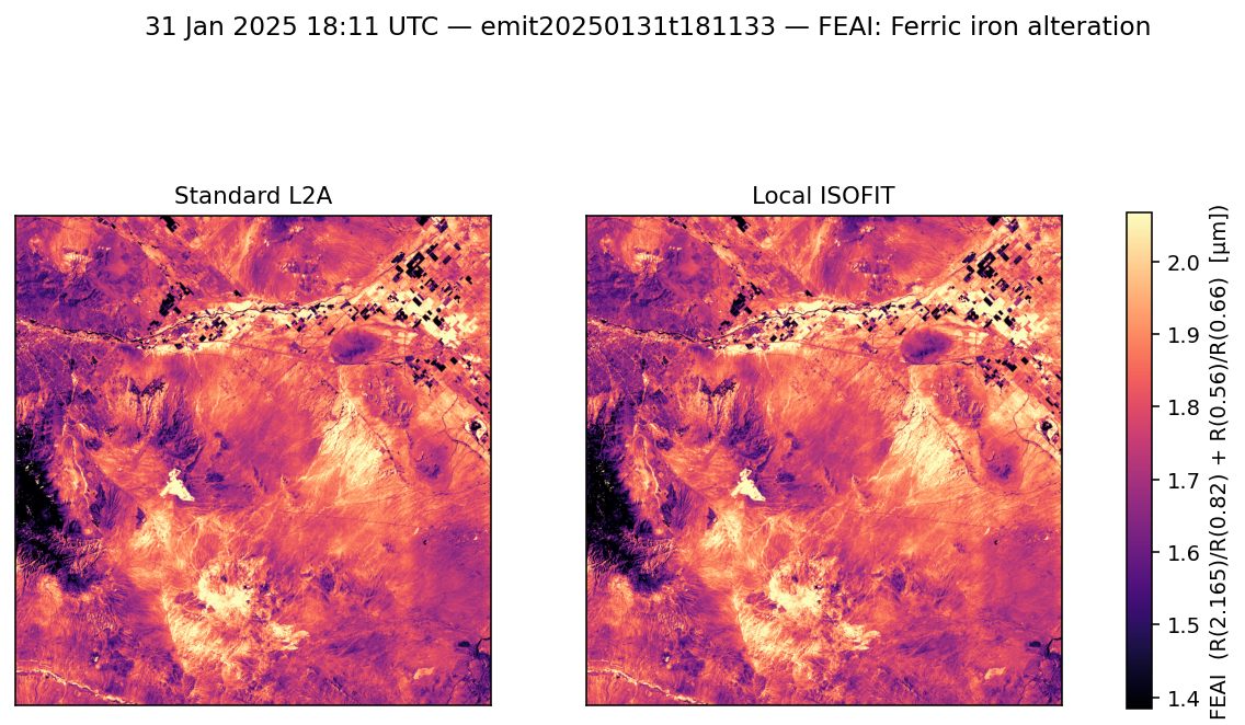
FEI_simple — Ferrous iron
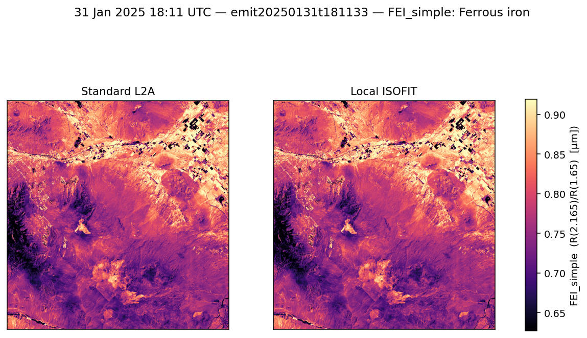
CLAY_TM — Generic clay (TM5/TM7 analog)
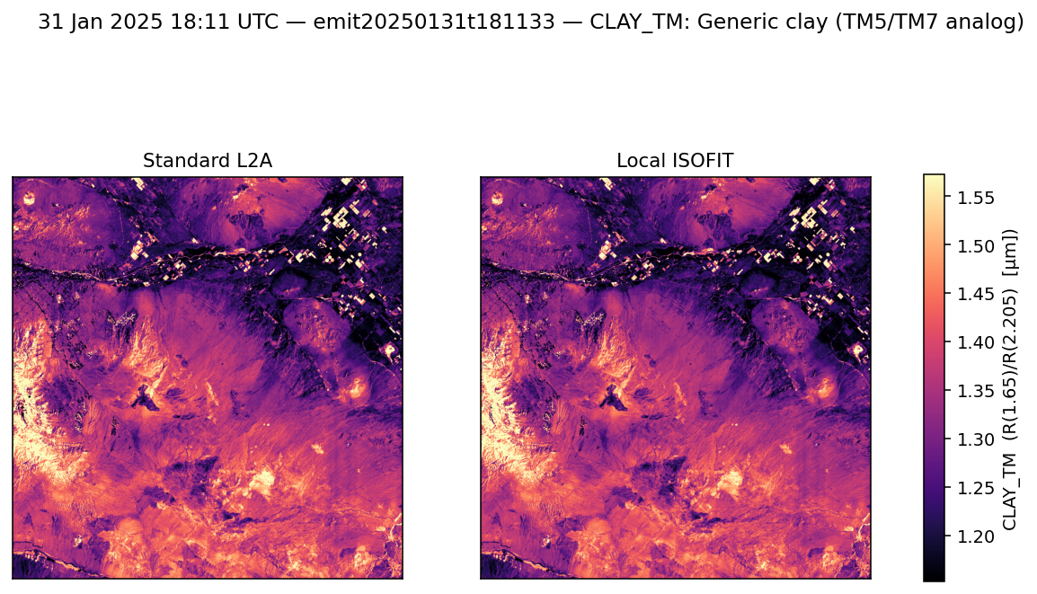
CLAI — Argillic alteration (alunite/kaolinite)
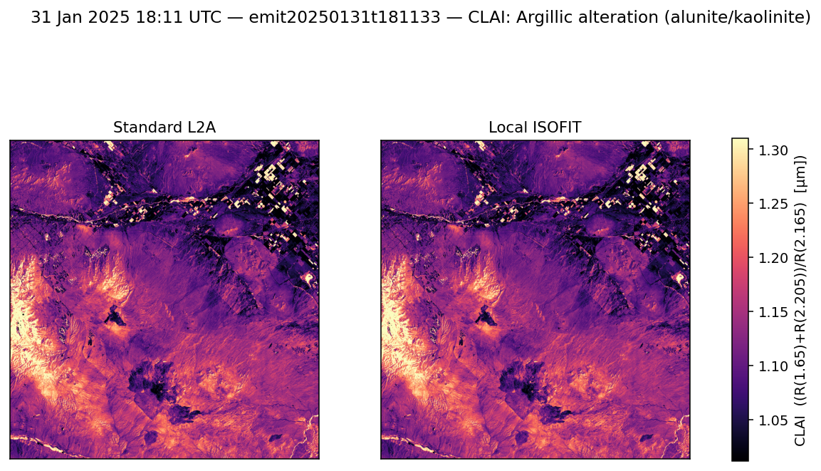
ALI — Alunite (Ninomiya)
KAI1 — Kaolinite slope
KLI — Kaolinite doublet
KAI3 — Kaolinite (alt 3-band)

OHI — OH-bearing minerals
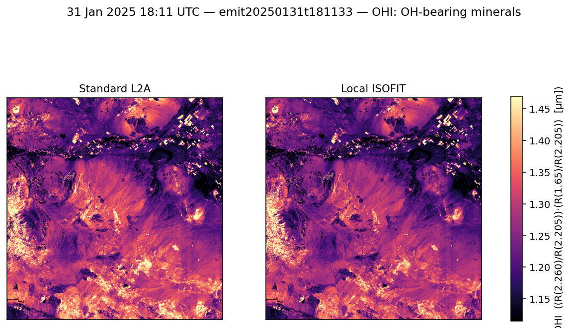
OHI3 — OH near 2.17 µm
CLI — Calcite
DOLI — Dolomite
MGAI — Mg-OH/chlorite/epidote
MONI — Montmorillonite
PRAI — Propylitic alteration
Tier 3 — High Cloud Fraction Not Included in Processing 9 scenes
Tier 4 — Missing Data Not Included in Processing 2 scenes
5. Discussion
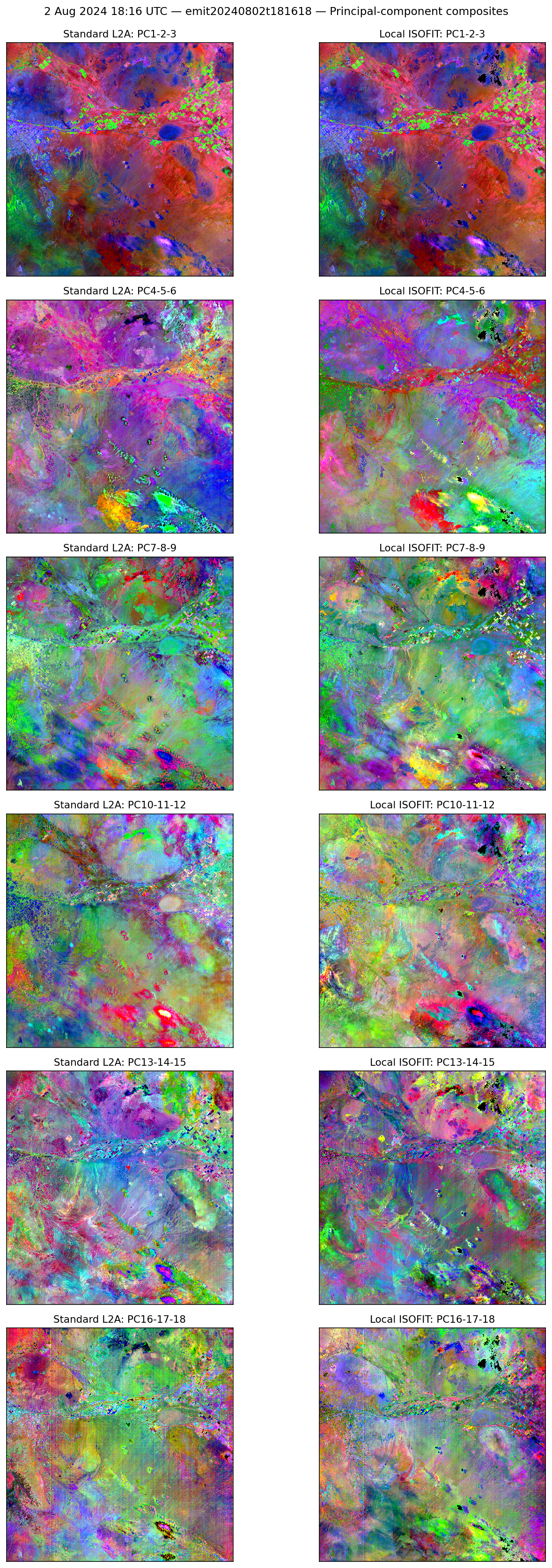
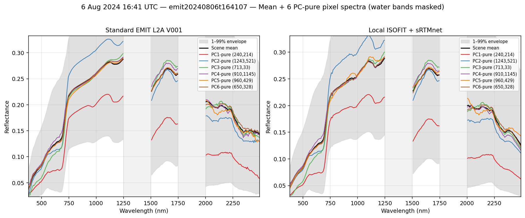
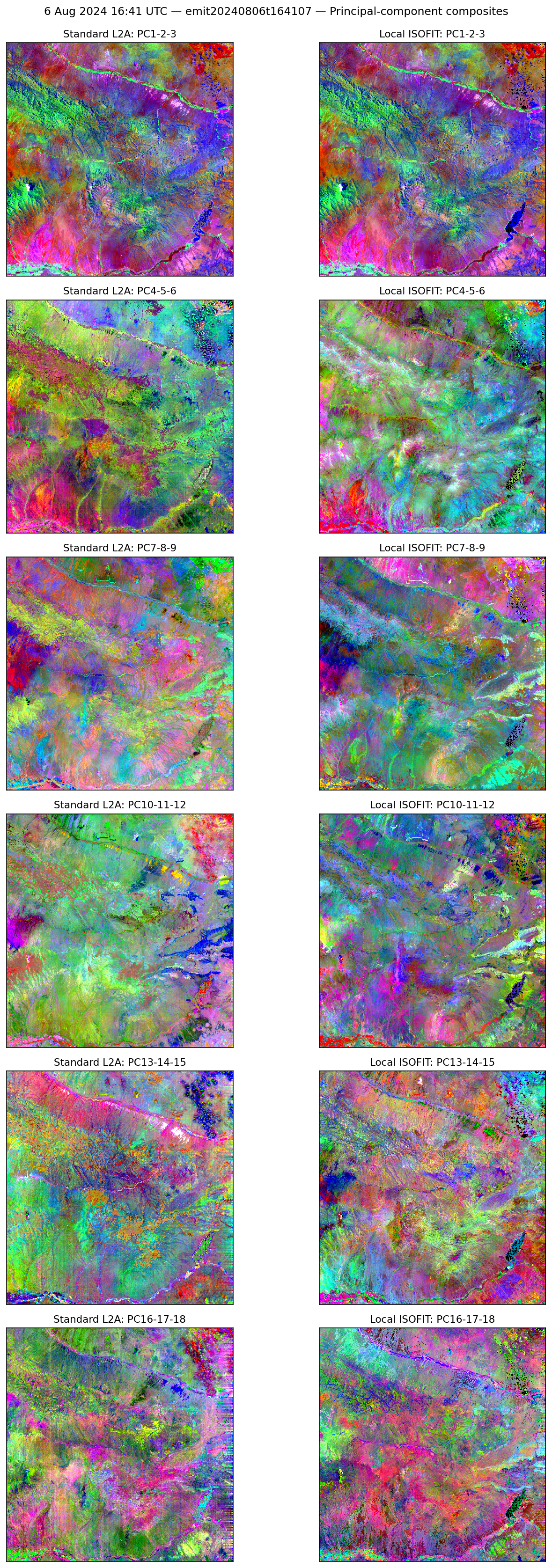
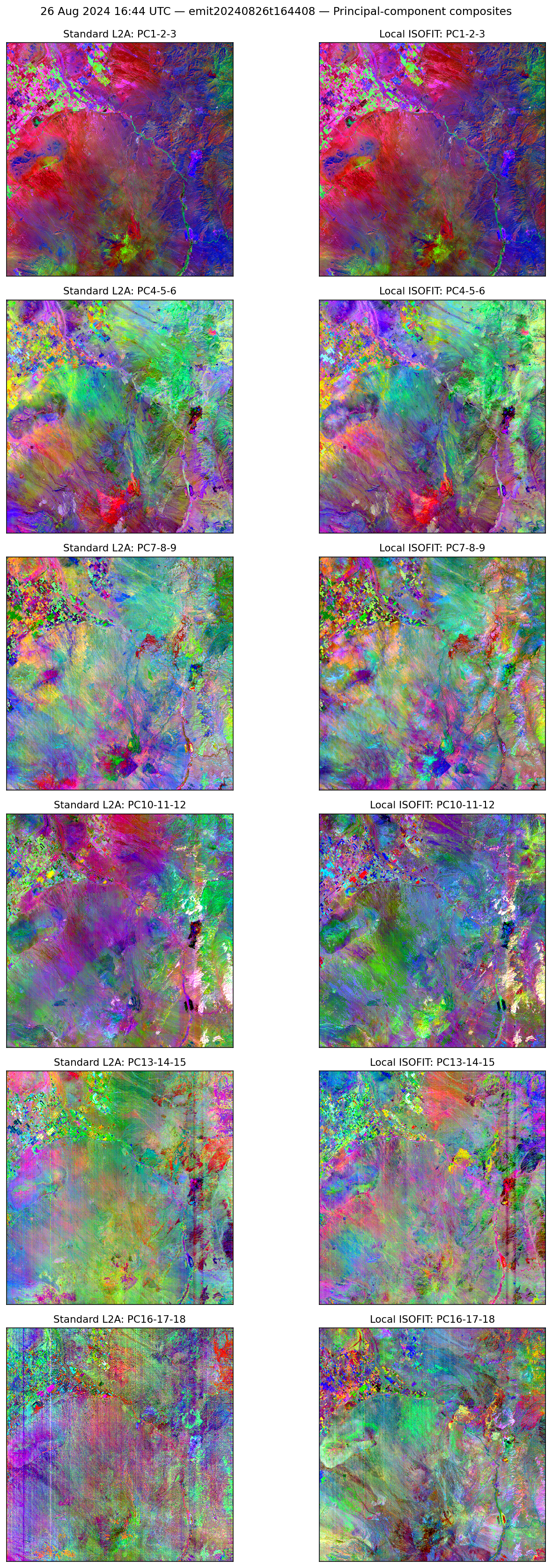
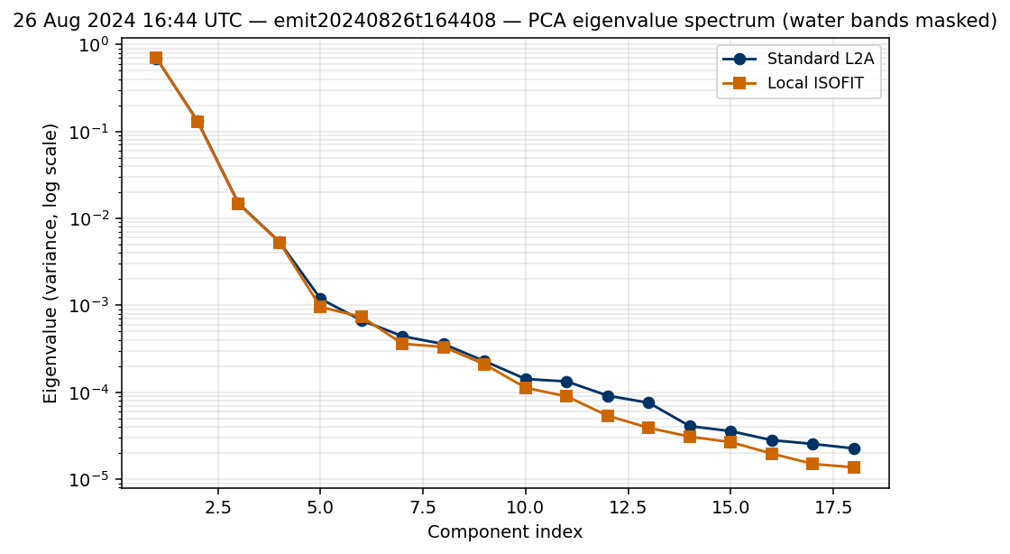
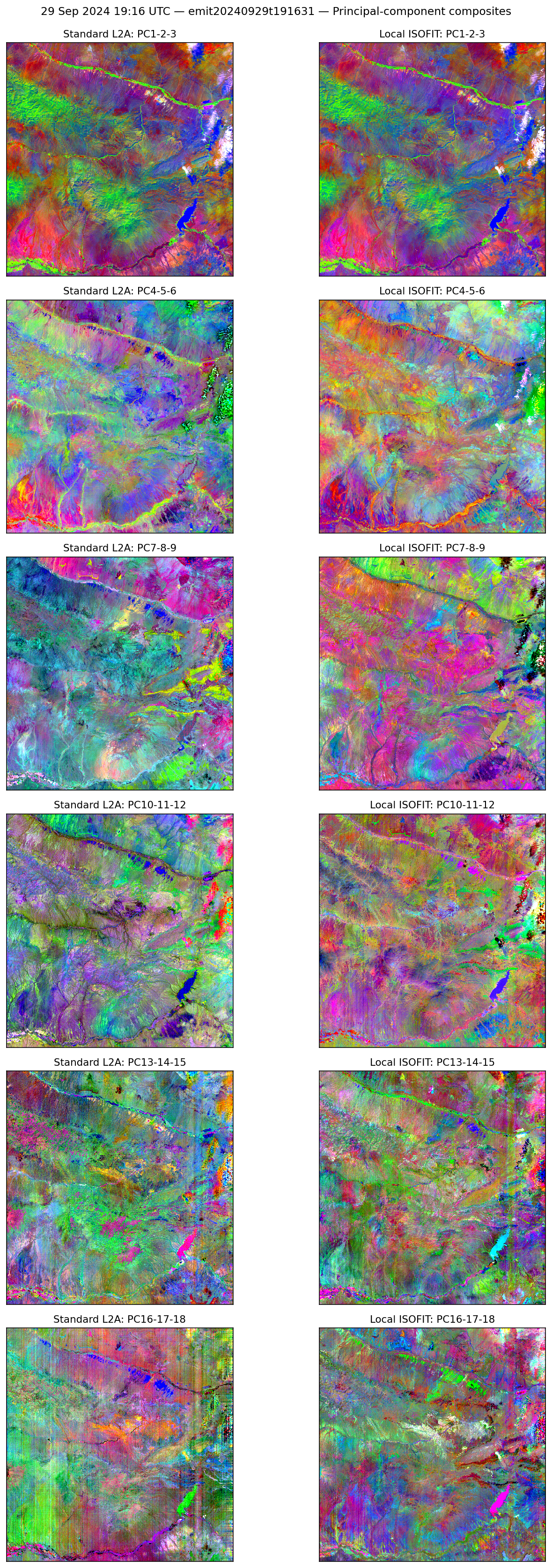
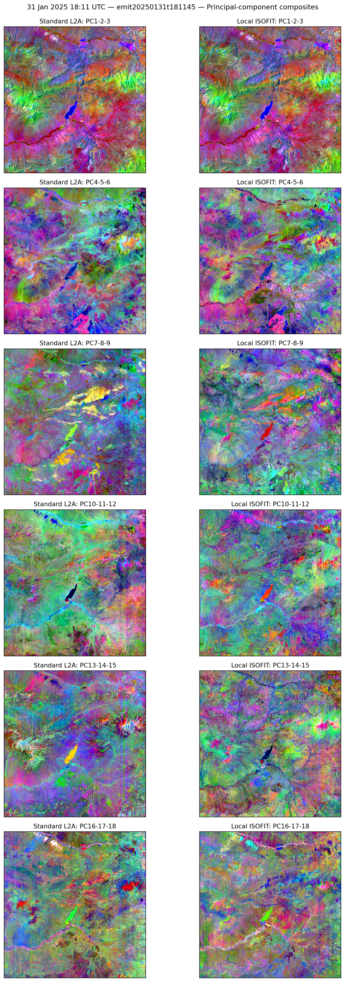
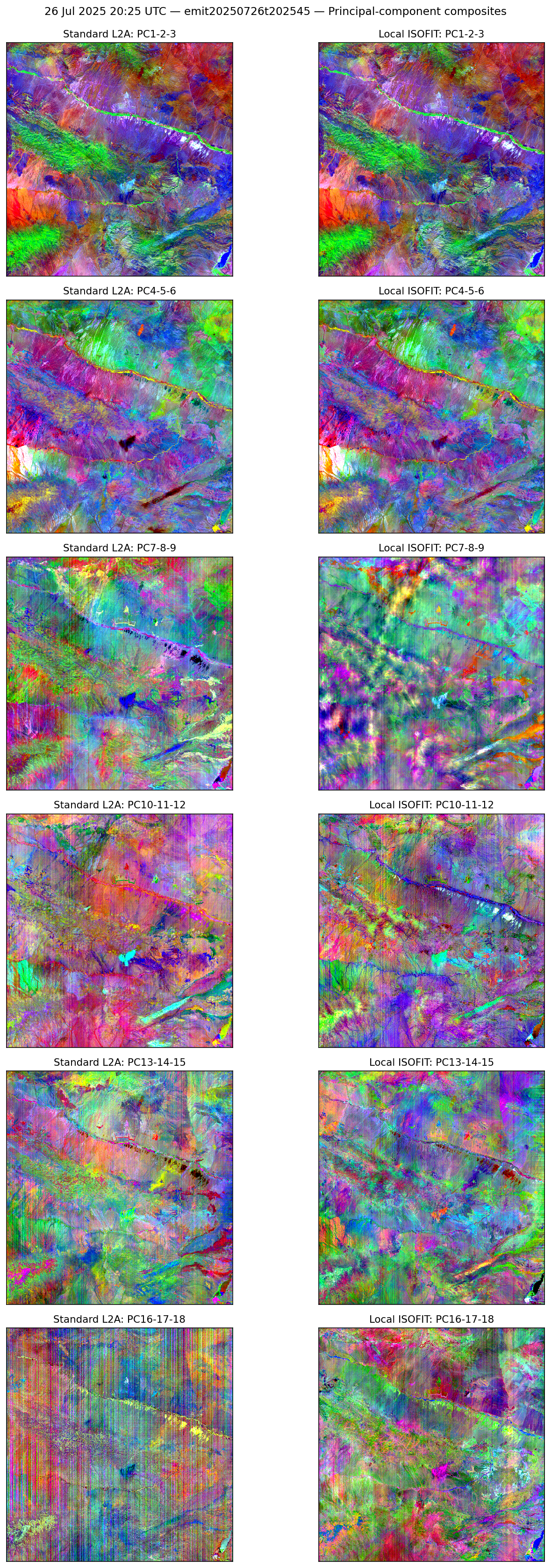
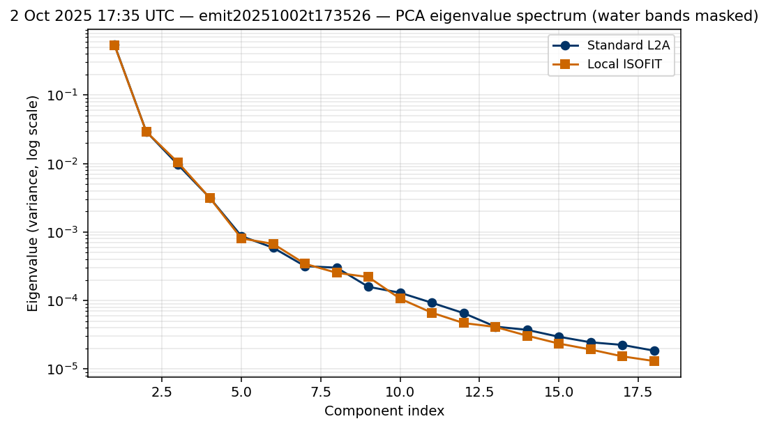
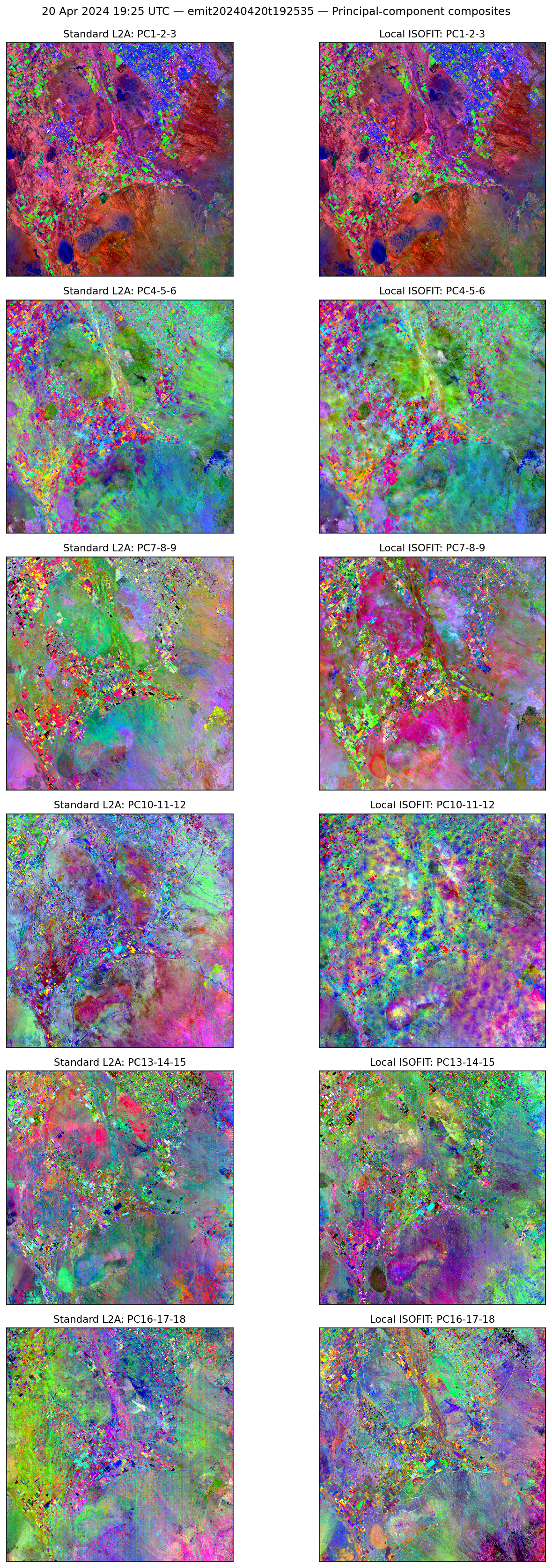
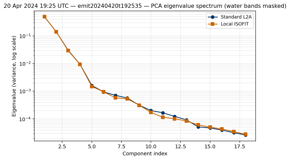
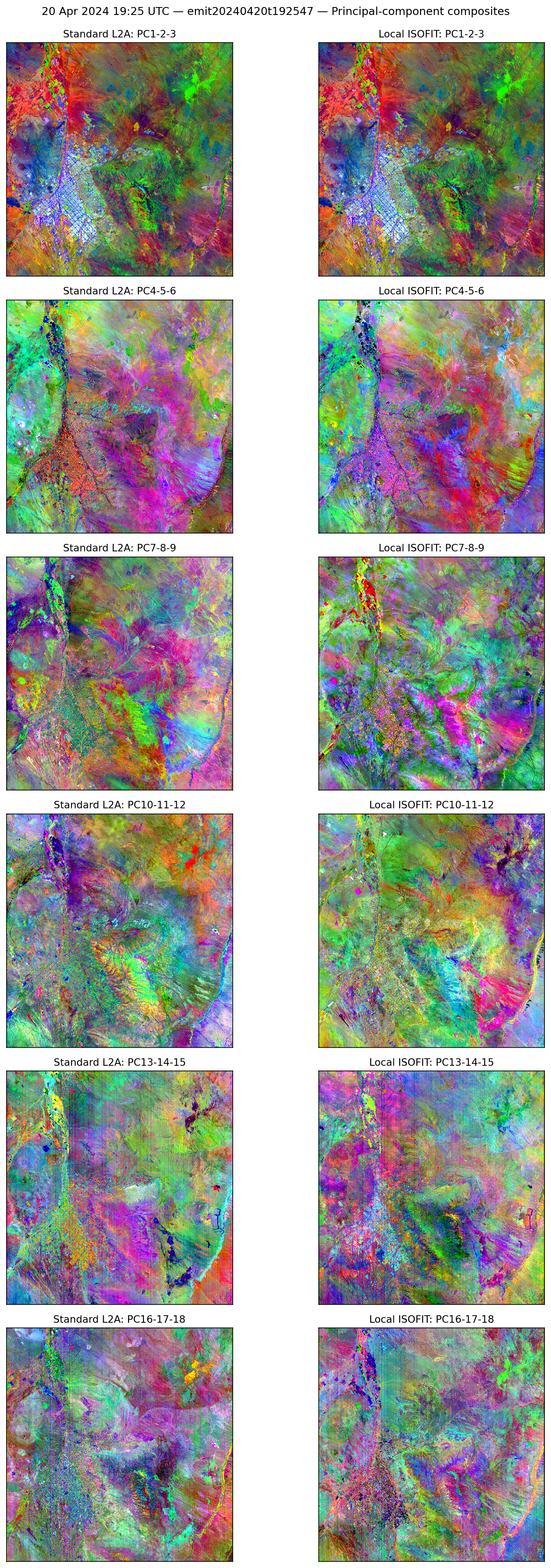
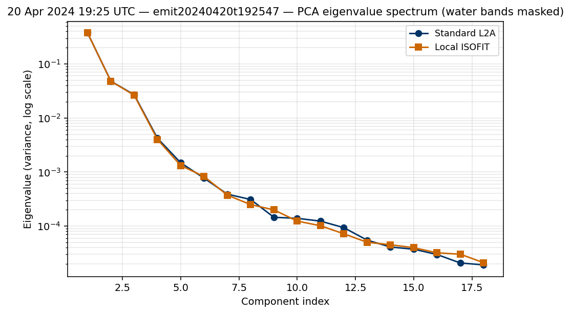
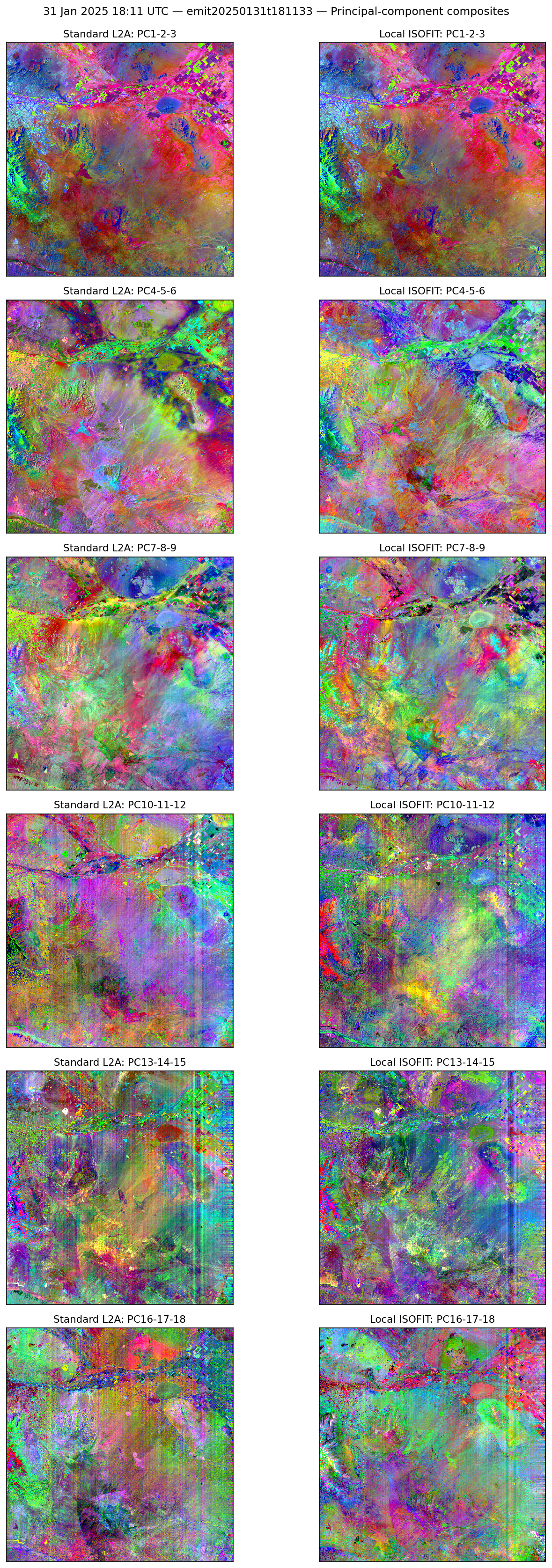
Across all scenes the true-color renders are visually indistinguishable: both retrievals flatten the atmospheric path radiance and recover surface color contrast. The PC-pure spectra agree closely on broad continuum shape but show systematic differences at the edges of the masked water regions — exactly the wavelengths where MODTRAN and the sRTMnet emulator differ most. The eigenvalue spectra are nearly parallel in their leading components but diverge in the tail, where atmospheric residuals live.
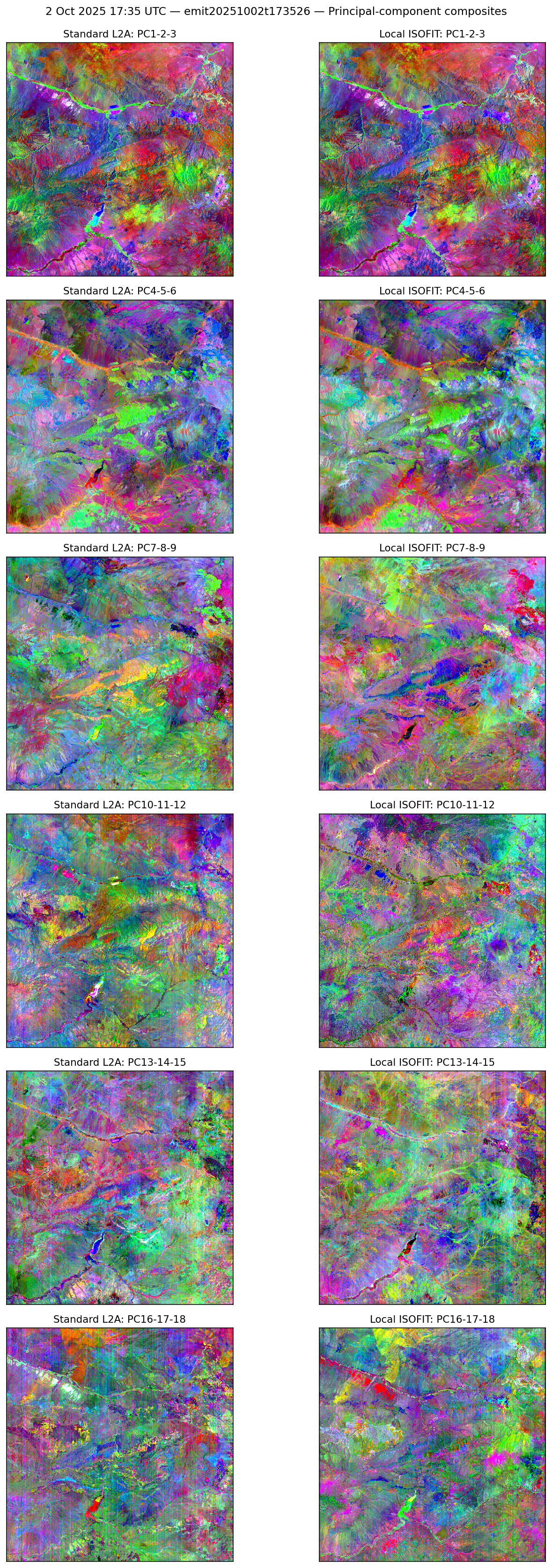
That divergence is informative. A perfect atmospheric correction would push residual covariance toward isotropic noise — a flat tail in log-eigenvalue space. Curvature in the tail indicates structured residuals that PCA can latch onto. We use that curvature, together with the higher-order PC composites, as a quick visual diagnostic of atmospheric-correction quality without ever needing ground truth.
Neither retrieval is "ground truth" — both are model-driven inversions of the same radiance with different RT engines and surface configurations. Their agreement is evidence the open-source path is operationally viable; it is not a validation against in-scene spectroradiometer measurements.
6. Reproducibility
All figures here are generated by a single self-contained Python script
(digital_whitepaper/build_whitepaper.py) that loads the standard L2A
from the LP DAAC NetCDF, the local ISOFIT cube via the spectral ENVI reader,
applies the water-band mask, fits PCA on a 80,000-pixel subsample, picks PC-pure pixels,
and renders all comparison figures. The local ISOFIT runs are produced by:
# EMIT scene → ISOFIT 3.7.x + sRTMnet
from isofit.utils.apply_oe import apply_oe
apply_oe(
    input_radiance     = "<flight>_rdn",
    input_loc          = "<flight>_loc",
    input_obs          = "<flight>_obs",
    sensor             = "emit",
    surface_path       = "data/surface/emit_surface.mat",
    emulator_base      = ".../sRTMnet_v100.h5",
    segmentation_size  = 40,
    presolve           = True,
    analytical_line    = True,
)
References
[1] Brodrick, P. G., Thompson, D. R., Garay, M. J., Giuliano, J., Green, R. O., et al. (2025). Improved Atmospheric Correction for Remote Imaging Spectroscopy Missions with Accelerated Optimal Estimation. Jet Propulsion Laboratory.
[2] Thompson, D. R., Natraj, V., Green, R. O., Helmlinger, M. C., Gao, B.-C., & Eastwood, M. L. (2018). Optimal Estimation for Imaging Spectrometer Atmospheric Correction. Remote Sensing of Environment, 216, 355–373.
[3] Connelly, D. S., Thompson, D. R., Mahowald, N. M., et al. (2021). The EMIT Mission Information Yield for Mineral Dust Radiative Forcing. Remote Sensing of Environment, 258, 112380.
[4] Berk, A., et al. (1998). MODTRAN cloud and multiple scattering upgrades with application to AVIRIS. Remote Sensing of Environment, 65(3), 367–375.
[5] Vermote, E. F., Tanré, D., Deuzé, J. L., Herman, M., & Morcrette, J. J. (1997). 6S: An Overview. IEEE Trans. Geosci. Remote Sens., 35(3), 675–686.
[6] Brodrick, P. G., Thompson, D. R., & Green, R. O. (2021). sRTMnet: Neural-network emulation of 6S for hyperspectral atmospheric correction. Remote Sensing of Environment.
[7] Adler-Golden, S. M., Berk, A., Bernstein, L. S., et al. (1999). FLAASH. Proc. AVIRIS Workshop.
[8] Basener, W. (2023). Gaussian Process and Deep Learning Atmospheric Correction. Remote Sensing 15(3), 649. mdpi.com/2072-4292/15/3/649
[9] Ninomiya, Y. (2003). A stabilized vegetation index and several mineralogic indices defined for ASTER VNIR and SWIR data. IGARSS 2003.
[10] Rowan, L. C., & Mars, J. C. (2003). Lithologic mapping in the Mountain Pass, California area using ASTER data. Remote Sensing of Environment 84(3), 350–366.
[11] Green, R. O., et al. (2020). The Earth Surface Mineral Dust Source Investigation. IEEE Aerospace Conference.
[12] EMIT L2A Algorithm Theoretical Basis Document, NASA JPL, V001.